© M.K. Atakishiyeva et al., Published by EDP Sciences 2019

Introduction

In the present work, we discuss some additional findings concerning algebraic properties of the discrete (finite) Fourier transform (DFT) raising and lowering difference operators, recently introduced in [1, 2]. 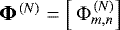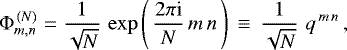Perhaps, it is worthwhile to recall first that the DFT based on points N is represented by an N × N unitary symmetric matrix ${\text{Φ}}^{(N)}=[{\text{Φ}}_{m,n}^{(N)}]$ with entries $${\Phi }_{m,n}^{(N)}=\frac{1}{\sqrt{N}}\exp (\frac{2\pi \text{i}}{N}mn)\equiv \frac{1}{\sqrt{N}}{q}^{mn},$$ $$q:=\exp (2\pi \text{i}/N),m,n\in \{0,1,\dots ,N-1\}.$$(1)

This matrix Φ^(N) was introducedby Sylvester [3] in 1867 and frequently referred to as Schur’s matrix.

Given a complex valued vector y⃗ with components ${\left\{y_k\right\}}_{k=0}^{N-1}$, one can compute another vector z⃗ with components 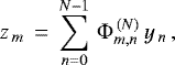$$z_m={\sum }_{n=0}^{N-1}{\Phi }_{m,n}^{(N)}{y}_n,$$(2)

referred to as the DFT of the vector y⃗. Those vectors f⃗^{( k)}, which are solutions of the standard equations 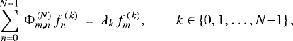$${\sum }_{n=0}^{N-1}{\Phi }_{m,n}^{(N)}{f}_n^{(k)}={\lambda }_k{f}_m^{(k)},k\in \{0,1,\dots ,N-1\},$$(3)

then represent eigenvectors of the DFT operator Φ^(N), associated with the eigenvalues λ_k. Since the fourth power of Φ^(N) is the unit operator, the only four distinct eigenvalues among λ_k’s are ± 1 and ± i.

An important aspect to observe at this point is that the same type of degeneracy of the eigenvalues is characteristic of the continuous counterpart of the DFT, the Fourier integral transform (FIT) that is also a unitary operator of order 4 with the same eigenvalues ± 1 , ± i. Note also that it is customary to reduce the problem of deriving the eigenfunctions of FIT to that of finding a differential operator of the lowest order with distinct eigenvalues, that commutes with the FIT operator and therefore has the same set of eigenfunctions as the FIT operator. Such differential operator was found to be a second-order differential number operator $$N=\frac{1}{2}(x^2-\frac{d^2}{d{x}^2}-1)$$(4)

which has distinct eigenvalues λ_n := n, n = 0, 1, 2, … , associated with the eigenfunctions 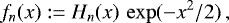$$f_n(x):=H_n(x)\exp (-x^2/2),$$(5)

where H_n(x) are the Hermite polynomials [4]. Thus in this way not only the eigenfunctions of the FIT are found, but their degeneracies are lifted by enumerating those eigenfunctions with the aid of the distinct eigenvalues λ_n = n of the number operator N. Note that the functions f_n(x) are usually referred to as Hermite functions in the mathematical literature and, properly normalized, they represent the wave functions of the linear harmonic oscillator in non-relativistic quantum mechanics [5].

So, an attempt has been made in [1] to find, in complete analogy with the case of IFT operator, such an operator with distinct eigenvalues that commutes with the DFT operator Φ^(N) . Since from the outset it was evident that this required operator cannot be any differential operator of a finite order, it was proposed to construct first two difference lowering and raising operators b _N and $b_N^{\text{†}}$ with the aid of the standard intertwining relations $$b_N{\text{Φ}}^{(N)}=\text{i}{\text{Φ}}^{(N)}{b}_N,b_N^{\text{†}}{\text{Φ}}^{(N)}=-\text{i}{\text{Φ}}^{(N)}{b}_N^{\text{†}},N\ge 3,$$(6)

with the DFT operator Φ^(N). Then it is straightforward to verify, by using definition (6), that a discrete number operator, defined as a difference operator of the form $$N^{(N)}:=b_N^{\text{†}}{b}_N,$$(7)

does commute with the DFT operator Φ^(N). Therefore, it was conjectured in [1] that the eigenvalues of the discrete number operator $N^{(N)}$, based on an arbitrary number of points N, are represented by distinct non-negative numbers and the corresponding eigenvectors f⃗ _k , 0 ≤ k ≤ N − 1, can be successively defined, with the aid of the raising operator $b_N^{\text{†}}$, as $$f_{j+1}=\frac{1}{{\lambda }_{j+1}^{1/2}}{b}_N^{\text{†}}{f}_j,0\le j\le N-2,$$(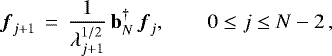8)

starting with the lowest eigenvector f⃗₀, which is found as a solution of the difference equation $$b_N{f}_0=0.$$(9)

In order to test the consistency of this approach to finding eigenfunctions and eigenvalues of the DFT operator Φ^(N) , the particular case of the 5-dimensional DFT was studied in detail in [6]. It was confirmed that the eigenvalues of the discrete number operator $N^{(5)}$ are represented by distinct non-negative numbers and the corresponding eigenvectors f⃗ _k , 0 ≤ k ≤ 4, can be successively defined with the aid of the raising operator $b_5^{\text{†}}$ and the lowest eigenvector f⃗₀, which is found as a solution of the difference equation b₅ f⃗₀ = 0.

The purpose of this presentation is to discuss some novel findings concerning algebraic properties of the N-dimensional DFT lowering and raising difference operators b_N and $b_N^{\text{†}}$. In particular, we evaluate in the next Section 2 the rank of lowering difference operator b _N (which is the same as the rank of the raising operator $b_N^{\text{†}}$) for an arbitrary dimension N. It turns out the rank of the b_N is equal to N − 1 for odd dimensions N, whereas it is equal to N − 2 for even dimensions N. This proves that the discrete number operator $N^{(N)}$ has a distinct spectrum only for odd dimensions N; the corresponding eigenvectors in all these cases can be successively constructed with the aid of (8) and (9). As for even dimensions N, this means that in those cases the discrete number operator $N^{(N)}$ has two repeated zero eigenvalues and one should therefore look for a non-standard way of finding the eigenvectors of the $N^{(N)}$ and relevantly ordering them. In Section 3, it is shown that this heretofore undetected distinction between DFTs based on odd and even points N is very consistentwith the well-known formula [7, 8] for the multiplicities of the eigenvalues, associated with the N-dimensional DFT operator Φ^(N). Finally, in Section 4, we put forward a general algorithm for constructing the eigenvectors of the discrete number operators $N^{(N)}$, that avoids the above-mentioned pitfalls in the structure of each even-dimensional case N = 2L.

N-dimensional raising and lowering operators

Algebraic properties of the N-dimensional DFT lowering b_N and raising $b_N^{\text{†}}$ difference operators were broached in [2] by the first two authors of this presentation. The development is continued here. In particular, in this section we extend those results by evaluating the rank of the operators b _N and $b_N^{\text{†}}$ for an arbitrary dimension N and demonstrating that the characteristic equations for those operators have a particular ‘cyclic’ form.

The N-dimensional lowering difference operator is represented by the N × N matrix 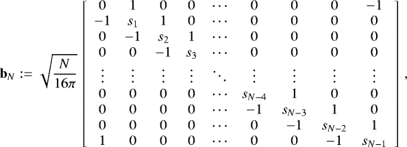$$b_N:=\sqrt{\frac{N}{16\pi }}\left[\begin{array}{ccccccccc}0& 1& 0& 0& \cdots & 0& 0& 0& -1\\ -1& s_1& 1& 0& \cdots & 0& 0& 0& 0\\ 0& -1& s_2& 1& \cdots & 0& 0& 0& 0\\ 0& 0& -1& s_3& \cdots & 0& 0& 0& 0\\ ⋮& ⋮& ⋮& ⋮& \ddots & ⋮& ⋮& ⋮& ⋮\\ 0& 0& 0& 0& \cdots & s_{N-4}& 1& 0& 0\\ 0& 0& 0& 0& \cdots & -1& s_{N-3}& 1& 0\\ 0& 0& 0& 0& \cdots & 0& -1& s_{N-2}& 1\\ 1& 0& 0& 0& \cdots & 0& 0& -1& s_{N-1}\end{array}\right],$$(10)

where we introduced for brevity 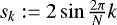$s_k:=2\sin \frac{2\pi }{N}k$, 0 ≤ k ≤ N − 1, and N is an arbitrary positive integer, N ≥ 3.

Notice that the matrix in (10) is traceless, because one checks easily that 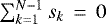${\sum }_{k=1}^{N-1}{s}_k=0$. Also, since s_N−k = − s_k by definition of the parameterss_k, the diagonal elements of the matrix in (10) are of the form $$\begin{array}{l}\{0,s_1,s_2,\dots ,s_{L-1},0,-s_{L-1},\dots ,-s_2,-s_1\},N=2L,\\ \{0,s_1,s_2,\dots ,s_L,-s_L,\dots ,-s_2,-s_1\},N=2L+1,\end{array}$$(11)

for even andodd dimensions N, respectively. This means that the operator b_N depends only on the L independent parameters {s₁, s₂, …, s_L} if N = 2L + 1 and on the L − 1 parameters {s₁ , s₂ , … , s_L−1} if N = 2L.

The matrix b_N is noninvertible (singular) and its rank is different for the even and odd dimensions N. This can be shown in the following way.

We recall first that the space spanned by the rows (columns) of a matrix A is called the row (column) space of A; its dimension is called the row (column) rank. The rank of a matrix equals the row (column) rank [9]. There are simple procedures available for finding bases for the row and column spaces of a matrix.

To find a basis of the row (column) space of a matrix A, use elementary row (column) operations to put A in reduced row (column) echelon form. Discard any zero rows (columns); then the remaining rows (columns) will form a basis of the row (column) space of A (see, for example, pages 41, 44, 49 and 127 in [10]).

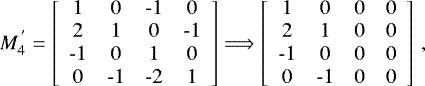
So, let us begin with examining the matrix 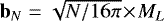$b_N=\sqrt{N/16\pi }\text{}\times \text{}{M}_L$ for odd N = 2L + 1, L ≥ 1, where the matrix M_L is $$M_L:=\left[\begin{array}{ccccccccccc}0& 1& 0& 0& \cdots & 0& 0& 0& \cdots & 0& -1\\ -1& s_1& 1& 0& \cdots & 0& 0& 0& \cdots & 0& 0\\ 0& -1& s_2& 1& \cdots & 0& 0& 0& \cdots & 0& 0\\ 0& 0& -1& s_3& \cdots & 0& 0& 0& \cdots & 0& 0\\ ⋮& ⋮& ⋮& \ddots & \ddots & \ddots & ⋮& ⋮& ⋮& ⋮& ⋮\\ 0& 0& \cdots & 0& -1& s_L& 1& 0& \cdots & 0& 0\\ 0& 0& \cdots & 0& 0& -1& -s_L& 1& \cdots & 0& 0\\ ⋮& ⋮& ⋮& ⋮& ⋮& ⋮& \ddots & \ddots & \ddots & ⋮& ⋮\\ 0& 0& \cdots & 0& 0& 0& \cdots & -1& -s_3& 1& 0\\ 0& 0& \cdots & 0& 0& 0& \cdots & 0& -1& -s_2& 1\\ 1& 0& \cdots & 0& 0& 0& \cdots & 0& 0& -1& -s_1\end{array}\right].$$(12)

By elementary column operations one may cast the matrix M_L into the form $$M_L^{\text{'}}=\left[\begin{array}{ccccccccccc}\hfill 1\hfill & \hfill 0\hfill & \hfill 0\hfill & \hfill \cdots \hfill & \hfill 0\hfill & \hfill 0\hfill & \hfill 0\hfill & \hfill \cdots \hfill & \hfill 0\hfill & \hfill -1\hfill & \hfill 0\hfill \\ \hfill s_1\hfill & \hfill 1\hfill & \hfill 0\hfill & \hfill \cdots \hfill & \hfill 0\hfill & \hfill 0\hfill & \hfill 0\hfill & \hfill \cdots \hfill & \hfill 0\hfill & \hfill 0\hfill & \hfill -1\hfill \\ \hfill -1\hfill & \hfill s_2\hfill & \hfill 1\hfill & \hfill \cdots \hfill & \hfill 0\hfill & \hfill 0\hfill & \hfill 0\hfill & \hfill \cdots \hfill & \hfill 0\hfill & \hfill 0\hfill & \hfill 0\hfill \\ \hfill 0\hfill & \hfill -1\hfill & \hfill s_3\hfill & \hfill \cdots \hfill & \hfill 0\hfill & \hfill 0\hfill & \hfill 0\hfill & \hfill \cdots \hfill & \hfill 0\hfill & \hfill 0\hfill & \hfill 0\hfill \\ \hfill ⋮\hfill & \hfill ⋮\hfill & \hfill \ddots \hfill & \hfill \ddots \hfill & \hfill \ddots \hfill & \hfill ⋮\hfill & \hfill ⋮\hfill & \hfill ⋮\hfill & \hfill ⋮\hfill & \hfill ⋮\hfill & \hfill ⋮\hfill \\ \hfill 0\hfill & \hfill \cdots \hfill & \hfill 0\hfill & \hfill -1\hfill & \hfill s_L\hfill & \hfill 1\hfill & \hfill 0\hfill & \hfill \cdots \hfill & \hfill 0\hfill & \hfill 0\hfill & \hfill 0\hfill \\ \hfill 0\hfill & \hfill \cdots \hfill & \hfill 0\hfill & \hfill 0\hfill & \hfill -1\hfill & \hfill -s_L\hfill & \hfill 1\hfill & \hfill \cdots \hfill & \hfill 0\hfill & \hfill 0\hfill & \hfill 0\hfill \\ \hfill ⋮\hfill & \hfill ⋮\hfill & \hfill ⋮\hfill & \hfill ⋮\hfill & \hfill ⋮\hfill & \hfill \ddots \hfill & \hfill \ddots \hfill & \hfill \ddots \hfill & \hfill ⋮\hfill & \hfill ⋮\hfill & \hfill ⋮\hfill \\ \hfill 0\hfill & \hfill \cdots \hfill & \hfill 0\hfill & \hfill 0\hfill & \hfill 0\hfill & \hfill \cdots \hfill & \hfill -1\hfill & \hfill -s_3\hfill & \hfill 1\hfill & \hfill 0\hfill & \hfill 0\hfill \\ \hfill 0\hfill & \hfill \cdots \hfill & \hfill 0\hfill & \hfill 0\hfill & \hfill 0\hfill & \hfill \cdots \hfill & \hfill 0\hfill & \hfill -1\hfill & \hfill -s_2\hfill & \hfill 1\hfill & \hfill 0\hfill \\ \hfill 0\hfill & \hfill \cdots \hfill & \hfill 0\hfill & \hfill 0\hfill & \hfill 0\hfill & \hfill \cdots \hfill & \hfill 0\hfill & \hfill 0\hfill & \hfill -1\hfill & \hfill -s_1\hfill & \hfill 1\hfill \end{array}\right],$$(13)

which is almost in the column echelon form, except for the two elements equal to − 1 on the upper right corner of this matrix. But it is not hard to eliminate them by further elementary column operations over the last two columns, and bring $M_L^{\text{'}}$ into complete column echelon form. Indeed, let us add to the penultimate column in (13) its first column plus the last one, multiplied by the parameter s₁, to get $$\left[\begin{array}{ccccccccccc}1& 0& 0& \cdots & 0& 0& 0& \cdots & 0& 0& 0\\ s_1& 1& 0& \cdots & 0& 0& 0& \cdots & 0& 0& -1\\ -1& s_2& 1& \cdots & 0& 0& 0& \cdots & 0& -1& 0\\ 0& -1& s_3& \cdots & 0& 0& 0& \cdots & 0& 0& 0\\ ⋮& ⋮& \ddots & \ddots & \ddots & ⋮& ⋮& ⋮& ⋮& ⋮& ⋮\\ 0& \cdots & 0& -1& s_L& 1& 0& \cdots & 0& 0& 0\\ 0& \cdots & 0& 0& -1& -s_L& 1& \cdots & 0& 0& 0\\ ⋮& ⋮& ⋮& ⋮& ⋮& \ddots & \ddots & \ddots & ⋮& ⋮& ⋮\\ 0& \cdots & 0& 0& 0& \cdots & -1& -s_3& 1& 0& 0\\ 0& \cdots & 0& 0& 0& \cdots & 0& -1& -s_2& 1& 0\\ 0& \cdots & 0& 0& 0& \cdots & 0& 0& -1& 0& 1\end{array}\right].$$(14)

So, the next step is to add to the last column in (14) the second column plus the penultimate one, multiplied by the parameter s₂; this results in $$\text{See PDF for equation.}$$(15)

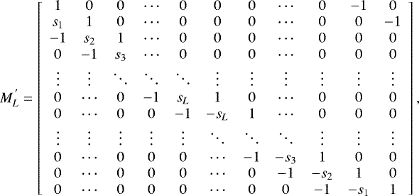
Let us emphasize that this form $M_L^{\text{'}\text{'}}$ of the initial matrix M_L contains the principal minor 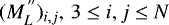${(M_L^{\text{'}\text{'}})}_{i,j},3\le i,j\le N$, of order N − 2 ≡ 2(L − 1) + 1, which results from the deletion of the first two rows and columns in (15), as indicated there by dashed line. This minor has a structure similar to the matrix $M_{L-1}^{\text{'}}$ in (13). One therefore may employ the same type of elementary column operations as above in order to move those two elements equal to − 1 in the last twocolumns in (15) another two rows down. Repeating those steps L − 1 times, one finally arrives at the form, which contains a principal minor of order 3 on its lower right corner; this minor has the same structure as $M_1^{\text{'}}$. It is plain that in the latter case 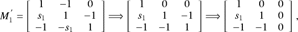$$M_1^{\text{'}}=\left[ccc1-10s_{1}1-1-1-s_{1}1\right]\Rightarrow \left[ccc100s_{1}1-1-1-11\right]\Rightarrow \left[ccc100s_{1}10-1-10\right],$$(16)

where we added the first column plus the third column, multiplied by s₁ , to the second column at the first step, and the second column to the third one at the second step. This means that the matrix M_L is finally reduced to the complete column echelon form of a lower triangular matrix, which has nonzero first N − 1 diagonal elements and only one zero element on its main diagonal. Hence det M_L = 0, rank M_L = N − 1 and the null space of the matrix M_L is one-dimensional. One therefore sees that the lowest eigenvector f⃗₀ of the discrete number operator $N^{(N)}$ is uniquely determined (up to normalization by a proper constant) by the equation b _N f⃗ ₀ = 0 and all other N − 1 eigenvectors f⃗ _j , 1 ≤ j ≤ N − 1 of the operator $N^{(N)}$, successively defined by (8), are linearly independent.

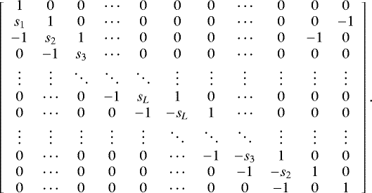
Turning now to the case of the matrix b_N with even N = 2L, L ≥ 2, it should be noted that the corresponding matrix in (10) for even N = 2L has almost the same structure as M_L in the odd case, except that only diagonal elements of those two matrices are different: as indicated in (11), there are two zero diagonal elements in the even case N = 2L and only one zero element in the odd caseN = 2L + 1. Therefore, onemay likewise employ the same inductive procedure in L as in the odd case N = 2L + 1 in order to move downwards those two elements equal to − 1 in the last two columns of the matrix 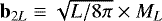$b_{2L}\equiv \sqrt{L/8\pi }\times M_L$, finally arriving at the form with aprincipal minor of order 4 on its lower right corner. This principal minor has the same structure as $M_4^{\text{'}}$, $$M_4^{\text{'}}=\left[cccc10-10210-1-10100-1-21\right]\Rightarrow \left[cccc10002100-10000-100\right],$$(17)

which is readily reduced to the echelon form, indicated in the above. One therefore checks easily that all even case matrices can be transformed, by elementary column operations, into the complete echelon form with two zero columns at the end. Thus in the even N = 2L case det b _N = 0, rank b _N = N − 2 and the null space of the matrix b_N is two-dimensional. This means that in the even case there are two linearly independent solutions of the difference equation b _N f⃗ ₀ = 0 for defining the lowest eigenvector of the discrete number operator $N^{(N)}$.

Let us draw attention now to the remarkable ‘cyclic’ properties of the lowering and raising difference operators b _N and $b_N^{\text{†}}$, which can be formulated in the following way. Recall first that the equation which is solved to find eigenvalues of N × N matrix M is usually interpreted as the equation for finding roots of the characteristic polynomial $$p_M(\lambda ):=\text{det}(\lambda I-M)={\lambda }^N+c_1{\lambda }^{N-1}+c_2{\lambda }^{N-2}+\cdots +c_{N-1}\lambda +c_N,$$(18)

where I is the N × N identity matrix and the coefficient c_k is ${(-1)}^k$ times the sum of the determinants of all of the principal k × k minors of M (note that by this definition c₁ = − trace(M) and $c_N={(-1)}^N\text{det}M$ ). The Cayley–Hamilton theorem then states that an N × N matrix M is annihilated by its characteristic polynomial (18), that is, $$p_M(M)=M^N+c_1{M}^{N-1}+c_2{M}^{N-2}+\cdots +c_{N-1}M+c_{N}I=0.$$(19)

It is plain that for a singular traceless matrix M the coefficients c₁ and c_N vanish. It turns out that for the particular traceless matrices of the form b _N and $b_N^{\text{†}}$ there are many more vanishing coefficients in the identity (19). The point is that from the defining intertwining relations (6) for the lowering and raising difference operators b _N and $b_N^{\text{†}}$ it follows at once that $${({\text{Φ}}^{(N)})}^{\text{†}}{b}_N{\text{Φ}}^{(N)}=\text{i}{b}_N,{({\text{Φ}}^{(N)})}^{\text{†}}{b}_N^{\text{†}}{\text{Φ}}^{(N)}=-\text{i}{b}_N^{\text{†}}.$$(20)

This means that if, for instance, b_Nf⃗ = λ f⃗ and λ≠ 0, then 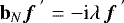$b_N{{\displaystyle \overrightarrow{f}}}^{\text{'}}=-\text{i}\lambda {{\displaystyle \overrightarrow{f}}}^{\text{'}}$, where the eigenvector ${{\displaystyle \overrightarrow{f}}}^{\text{'}}$ of the operator b_N is defined as ${{\displaystyle \overrightarrow{f}}}^{\text{'}}{≔(}^{(N)}{)}^{†}{\displaystyle \overrightarrow{f}}$. Hence, if the operator b _N has nonzero eigenvalue λ, associated with the eigenvector f⃗, then it has another eigenvalue −iλ, associated with the eigenvector ${\displaystyle \overrightarrow{f}}$, as well. Moreover, since the DFT operator Φ^(N) is of order 4, each nonzero eigenvalue λ is actually accompanied by the 3 other eigenvalues i^k λ , k = 1, 2, 3. Since the polynomial(z − λ)(z −iλ)(z + λ)(z + iλ) = z⁴ − λ⁴, one therefore concludes that in the characteristic equation (19) for the lowering operator b _N , N ≥ 5, the only nonzero coefficients are c₄, c₈, …, c_4k, where k := [N∕4] and the symbol [X] stands for the greatest integer in X. This characteristic equation can be thus written in the ‘cyclic’ form as $$b_N^N+c_4{b}_N^{N-4}+\dots +c_{4k}{b}_N^{N-4k}=(b_N^4-{\lambda }_1^4)(b_N^4-{\lambda }_2^4)\cdots (b_N^4-{\lambda }_k^4)b_N^l=0,$$(21)

where 0 ≤ l := N − 4k ≤ 3 and λ₁ , λ₂, …, λ_k are some constants.

To close this section, we recall here that the raising difference operator $b_N^{\text{†}}$ is the matrix transpose of the lowering difference operator b_N; hence the former operator has the same set of properties as the latter one: the vanishing determinant and trace, the same rank, distinct for even and odd dimensions N, and the same characteristic equation (21).

Multiplicities

As a starting point in this section, let us take the two so-called Chebyshev sets $$\{\sin t,\sin 2t,\dots ,\sin nt\},\{1,\cos t,\cos 2t,\dots ,\cos nt\},$$(22)

which are defined on intervals (0, π) and [0, π], respectively. These sets were employed in [7, 8] to give a simple proof of the explicit expressions for the multiplicities m_k (i^k ) of the eigenvalues i^k, 0 ≤ k ≤ 3, for the N-dimensional DFT operator Φ^(N) of the form: 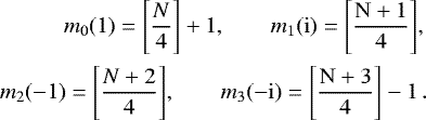$$\begin{array}{l}{m}_0(1)=[\frac{N}{4}]+1,m_1(\text{i})=[\frac{N+1}{4}],\\ m_2(-1)=[\frac{N+2}{4}],m_3(-\text{i})=[\frac{N+3}{4}]-1.\end{array}$$(23)

Note that the lowering b_N and raising $b_N^{\text{†}}$ difference operators, as well as their product, the discrete number operator $N^{(N)}$, do depend on the set of parameters {s₁, s₂, …, s_N−1}, which may be regarded as the particular case of the Chebyshev set of smooth functions taken at the distinct points t_k := 2πk∕N, 1 ≤ k ≤ (N − 1). Thus, the fact that this particular set of parameters {s₁, s₂, …, s_N−1} plays a key role in our study, is not accidental at all. But the real reason for mentioning here the formula (23) for multiplicities is the following.

The formula (23) had been known for a long time before the appearance of the above-mentioned papers [7 , 8 ]. Nevertheless, what seems to remain unnoticed is that this formula clearly points out the dissimilarity between ordering the even-dimensional eigenvectors and odd-dimensional eigenvectors of the DFT operator Φ^(N) . This can be argued in the following way.

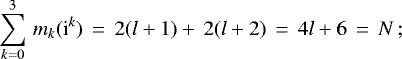
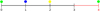
Imagine that one has a set of N marbles in 4 colors: m₀(1) green, m₁(i) blue, m₂(−1) yellow, and m₃(−i) red ones; the marbles of the same color are assumed for the moment to be identical. Also, there are boxes of various sizes with n + 1 compartments, which are consecutively labeled by 0, 1, 2, …, n. The question is how to select a box of minimal size in order to arrange in it, one by one, all the N marbles, taking into account that the green marbles may be placed only into compartments, marked as 0, 4, 8, … , blue marbles – into compartments, marked as 1, 5, 9, … , yellow marbles – into compartments, marked as 2, 6, 10, … , and red ones – into compartments 3, 7, 11, … .

To solve this rather simple combinatorial problem, observe that all odd dimensions N ≥ 3 can be divided intotwo sets as: $$a)N=3(\text{mod}4),\text{i}.\text{e}.,N=3+4l,l=0,1,2,3,\dots ,$$ $$m_0(1)=m_1(i)=m_2(-1)=l+1,m_3(-i)=l,$$ $${\sum }_{k=0}^3{m}_k({\text{i}}^k)=3(l+1)+l=4l+3=N;$$

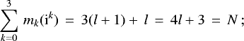
in particular, for N = 3 (i.e., l = 0) this set can be schematically depicted as $$b)N=5(\text{mod}4),\text{i}.\text{e}.,N=5+4l,l=0,1,2,3,\dots ,$$ $$m_0(1)=l+2,m_1(i)=m_2(-1)=m_3(-i)=l+1,$$ $${\sum }_{k=0}^3{m}_k({\text{i}}^k)=l+2+3(l+1)=4l+5=N;$$

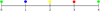
in particular, for N = 5 (i.e., l = 0) this set can be schematically depicted as

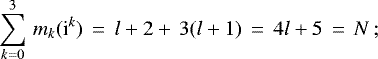
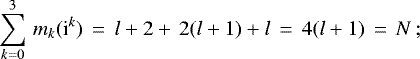
By the same token, all even dimensions N ≥ 4 can be divided into two sets of the form: $$a)N=4(\text{mod}4),\text{i}.\text{e}.,N=4+4l,l=0,1,2,3,\dots ,$$ $$m_0(1)=l+2,m_1(i)=m_2(-1)=l+1,m_3(-i)=l,$$ $${\sum }_{k=0}^3{m}_k({\text{i}}^k)=l+2+2(l+1)+l=4(l+1)=N;$$

in particular, for N = 4 (i.e., l = 0) this set can be schematically depicted as $$b)N=6(\text{mod}4),\text{i}.\text{e}.,N=6+4l,l=0,1,2,3,\dots ,$$ $$m_0(1)=l+2,m_1(i)=l+1,m_2(-1)=l+2,m_3(-i)=l+1,$$ $${\sum }_{k=0}^3{m}_k({\text{i}}^k)=2(l+1)+2(l+2)=4l+6=N;$$

in particular, for N = 6 (i.e., l = 0) this set can be schematically depicted as

Inspection of Figures 1–4 indicates that for each odd number N of marbles it is sufficient to use a box, which contains only N compartments in it; whilst in the case of all even numbers N of marbles one needs to use boxes with N + 1 compartments in them. Thus simply by examining the well-known equation (23) for the multiplicities of the eigenvalues for the N-dimensional DFT operator Φ^(N) one arrives at the same conclusions concerning essential differences between symmetry properties of the eigenvectors for the even- and odd-dimensional DFT operator, as we elaborated at the end of the previous section.

Fig. 1

Fig. 2

Eigenvectors for the even cases N=2L

It is evident now that for all even dimensions N = 2L there are multiple eigenvalues in the spectrum of the discrete number operator $N^{(2L)}$ and there is always a gap in the associated with them multiplicities (23) (see Figs. 3 and 4). Hence, it is not possible to employ the same conventional algorithm for finding the eigenvectors of the operator $N^{(2L)}$ as in the case of odd dimensions N = 2L + 1, when the all appropriate eigenvectors are successively constructed with the aid of the difference raising $b_N^{\text{†}}$ and lowering b_N operators via (8) and (9). However, it turns out that there is a more elaborate way of finding the eigenvectors for the $N^{(2L)}$, which enables one to surmount the above-mentioned obstacles in the structure of the each even-dimensional discrete number operator $N^{(2L)}$ and its spectrum.

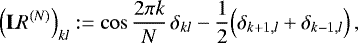
The key step in our approach towards finding the eigenvectors of the operator $N^{(2L)}$ is the use of certain properties of an additional lowering-raising operator LR^(N) of the form $${(L\text{}{R}^{(N)})}_{kl}:=\cos \frac{2\pi k}{N}{\delta }_{kl}-\frac{1}{2}({\delta }_{k+1,l}+{\delta }_{k-1,l}),$$(24)

where 0 ≤ k, l ≤ N − 1, δ_−1,l = δ_N−1,l and δ_N,l = δ_0,l. As detailed in Section 3 of [1], thus introduced operator LR^(N) anticommutes with the DFT operator Φ^(N), that is, $$L\text{}{R}^{(N)}{\text{Φ}}^{(N)}=-{\text{Φ}}^{(N)}L\text{}{R}^{(N)}.$$(25)

From (25) it follows at once that the action of the operator LR^(N) on the eigenvector f⃗ _k of the DFT operator Φ^(N) , associated with the eigenvalue i^k, 0 ≤ k ≤ 3, is a linear combination of the two eigenvectors f⃗_k−2 and f⃗ _k+2 of the DFT operator Φ^(N), i.e., 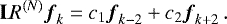$$L\text{}{R}^{(N)}{f}_k=c_1{f}_{k-2}+c_2{f}_{k+2}.$$(26)

That is why this operator is regarded as a double step lowering–raising difference operator and denoted by the symbol LR^(N) .

$$b_N=\sqrt{\frac{N}{16\pi }}[V^{\text{†}}-V+\text{i}(U^{\text{†}}-U)],b_N^{\text{†}}=\sqrt{\frac{N}{16\pi }}[V-V^{\text{†}}+\text{i}(U^{\text{†}}-U)],$$(27)

where U_k,l := q^kδ_k,l and V _k,l := δ_k,l+1 (see [1, 2]). The self-adjoint difference operator LR^(N) can be written in terms of these unitary operators U and V as 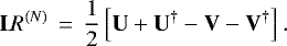$$L\text{}{R}^{(N)}=\frac{1}{2}[U+U^{\text{†}}-V-V^{\text{†}}].$$(28)

We are nowin a position to discuss an appropriate algorithm for finding the eigenvectors of the discrete number operator $N^{(2L)}$. Recall first that all even dimensions N ≥ 4 under study in this section can be divided into two subsets of dimensions N = 4 (mod 4) and N = 6 (mod 4). Moreover, all hierarchies of the eigenvectors of the $N^{(2L)}$ within the first subset have the same structure as in the case of N = 4 (see Fig. 3), whereas all sets of the eigenvectors from the second subset exhibit the same structure as in the case of N = 6 (see Fig. 4).

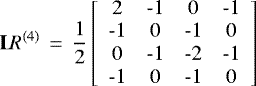
(a) Let us begin with examining the case of N = 4, when the lowering difference operator b₄ is represented by the 4 × 4 matrix, $$b_4=\frac{1}{2\sqrt{\pi }}\left[\begin{array}{ccccccccccccc}0& 1& 0& \$-1\$\text{ cr}\$-1\$& 2& 1& 0\text{ cr}0& \$-1\$& 0& 1\text{ cr}1& 0& \$-1\$& \$-2\$\text{ cr}\end{array}\right].$$(29)

As in the odd case with N = 2L + 1, the lowest eigenvector 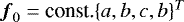$f_0=\text{const}.{\{a,b,c,b\}}^T$ is found as a solution of the difference equation b₄f⃗₀ = 0. Unlike the odd case with N = 2L + 1, this equation has two linearly independent solutions of the form 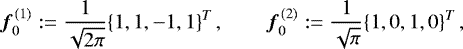$$f_0^{(1)}:=\frac{1}{\sqrt{2\pi }}{\{1,1,-1,1\}}^T,f_0^{(2)}:=\frac{1}{\sqrt{\pi }}{\{1,0,1,0\}}^T,$$(30)

and both of these solutions are eigenvectors of the DFT operator Φ⁽⁴⁾ , associated with the same eigenvalue i⁰ = 1. It is to be remarked that in this case one readily identifies that the second solution $f_0^{(2)}$ actually represents the last eigenvector f⃗₄ in the hierarchy of all eigenvectors of the discrete number operator $N^{(4)}$ (see Fig. 3), because it is annihilated also by the raising difference operator $b_4^{\text{†}}$, that is, $b_4^{\text{†}}{f}_0^{(2)}=0$. As for the first solution $f_0^{(1)}$, it may be usedto find the two remaining linearly independent eigenvectors of the discrete number operator $N^{(4)}$ as $$f_1:=\frac{1}{{\sqrt{\lambda }}_1}{b}_4^{\text{†}}{f}_0=\frac{1}{\sqrt{\pi }}{\{0,1,0,-1\}}^T,f_2:=\frac{1}{{\sqrt{\lambda }}_2}{b}_4^{\text{†}}{f}_1=\frac{1}{\sqrt{2\pi }}{\{-1,1,1,1\}}^T,$$(31)

where $f_0\equiv f_0^{(1)}$ and λ₁ = λ₂ = 2∕π. The 4 orthonormal vectors f⃗₀, f⃗₁, f⃗₂ and f⃗ ₄ thus form a complete set of the eigenvectors for the discrete number operator $N^{(4)}$, associated with the eigenvalues λ₀ = 0, λ₁ = λ₂ = 2∕π, λ₄ = 0, respectively.

It remains only to add that in this case with N = 4 there is no need to use the lowering-raising operator $$L\text{}{R}^{(4)}=\frac{1}{2}\left[\begin{array}{ccccccccccccc}2& \$-1\$& 0& \$-1\$\text{ cr}\$-1\$& 0& \$-1\$& 0\text{ cr}0& \$-1\$& \$-2\$& \$-1\$\text{ cr}\$-1\$& 0& \$-1\$& 0\text{ cr}\end{array}\right]$$(32)

in order to find the eigenvector f⃗₄ next to the gap in the set of all eigenvectors f⃗_k, 0 ≤ k ≤ 4, since from the very beginning this eigenvector surfaces as the second solution in (30) of the difference equation b ₄ f⃗ ₀ =0. However, as the consistency check of our approach to finding the eigenvectors of the discrete number operator $N^{(4)}$, one may verify that the operator LR⁽⁴⁾ does express the vector f⃗₄ in terms of the vector f⃗₂, i.e., over the above-mentioned gap, as 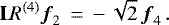$$L\text{}{R}^{(4)}{f}_2=-\sqrt{2}{f}_4.$$(33)

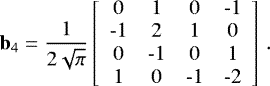
(b) In the case of N = 6 the lowering difference operator b₆ is represented by the 6 × 6 matrix, 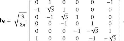$$b_6=\sqrt{\frac{3}{8\pi }}\left[\begin{array}{cccccc}0& 1& 0& 0& 0& -1\\ -1& \sqrt{3}& 1& 0& 0& 0\\ 0& -1& \sqrt{3}& 1& 0& 0\\ 0& 0& -1& 0& 1& 0\\ 0& 0& 0& -1& -\sqrt{3}& 1\\ 1& 0& 0& 0& -1& -\sqrt{3}\end{array}\right].$$(34)

Similar to the odd case with N = 2L + 1, the lowest eigenvector $f_0=\text{const}.{\{a,b,c,d,c,b\}}^T$ is found as a solution of the difference equation b₆f⃗₀ = 0. This equation has only one solution of the form $$f_0=\frac{1}{c_0}{\{1+\sqrt{3}(1+\sqrt{2}),1+\sqrt{2},1,1+\sqrt{2}-\sqrt{3},1,1+\sqrt{2}\}}^T,c_0=2\sqrt{\pi (2+\sqrt{2})},$$(35)

which represents at the same time the eigenvector of the DFT operator Φ⁽⁶⁾ , associated with the eigenvalue i ⁰ = 1. Since the rank of the difference raising operator $b_6^{\text{†}}$ is equal to 4, the next 4 linearly independent eigenvectors are then successively defined to be 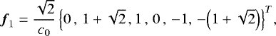$$f_1=\frac{\sqrt{2}}{c_0}{\{0,1+\sqrt{2},1,0,-1,-(1+\sqrt{2})\}}^T,$$(36) $$f_2=\frac{1}{\sqrt{3}{c}_0}{\{-2(1+\sqrt{2}),\sqrt{3}(1+\sqrt{2})-1,1+\sqrt{2}+\sqrt{3},2,1+\sqrt{2}+\sqrt{3},\sqrt{3}(1+\sqrt{2})-1\}}^T,$$(37) $$f_3=\frac{1}{\sqrt{3}{c}_0}{\{0,-1,1+\sqrt{2},0,-(1+\sqrt{2}),1\}}^T,$$(38) $$f_4=\frac{1}{3c_0}{\{2,-(1+\sqrt{2}+\sqrt{3}),\sqrt{3}(1+\sqrt{2})-1,2(1+\sqrt{2}),\sqrt{3}(1+\sqrt{2})-1,-(1+\sqrt{2}+\sqrt{3})\}}^T,$$(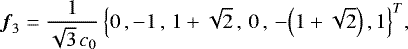39)

by using the conventional sequence of formulas (8). All these eigenvectors f⃗ _k , 1 ≤ k ≤ 4, are associated with the same eigenvalues λ_k = 9∕4π of the discrete number operator $N^{(6)}$; at the same time they are associated with the eigenvalues i^k of the DFT operator Φ⁽⁶⁾, respectively.

Observe that the subsequent action of the raising difference operator $b_6^{\text{†}}$ on the eigenvector f⃗₄ gives $$b_6^{\text{†}}{f}_4=-\frac{1}{2\sqrt{\pi }}{f}_1,$$(40)

which is consistent with the equation (23) for the multiplicities in the 6-dimensional case (see Fig. 4).

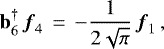
To find the last eigenvector f⃗₆ of the discrete number operator $N^{(6)}$, let us evaluate first $$L\text{}{R}^{(6)}{f}_4=-\frac{1+\sqrt{3}}{3\sqrt{2}{c}_0}{\{1-\sqrt{3}(1+\sqrt{2}),1+\sqrt{2},1,1+\sqrt{2}+\sqrt{3},1,1+\sqrt{2}\}}^T=:-g_6.$$(41)

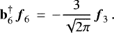
From (26) it follows that g⃗₆ = c₁f⃗₂ + c₂f⃗₆ and to define the first coefficient c₁ in this linear combination of the vectors f⃗₂ and f⃗ ₆ , one evaluates next that $$(f_6,f_2)=c_1(f_2,f_2)=\frac{\sqrt{2}(1+\sqrt{3})}{3\pi },c_1=\frac{1+\sqrt{3}}{3\sqrt{2}}.$$(42)

Consequently, $$c_2{f}_6=g_6-c_1{f}_2=\frac{c_1}{\sqrt{3}{c}_0}{\{\sqrt{3}-\sqrt{2}-1,1,-(1+\sqrt{2}),1+(1+\sqrt{2})\text{}\sqrt{3},-(1+\sqrt{2}),1\}}^T,$$(43)

from which it follows at once that c₂ = c₁ and $$f_6:=\frac{1}{\sqrt{3}{c}_0}{\{\sqrt{3}-\sqrt{2}-1,1,-(1+\sqrt{2}),1+(1+\sqrt{2})\text{}\sqrt{3},-(1+\sqrt{2}),1\}}^T.$$(44)

It is not hard to verify that thus defined vector f⃗ ₆ is the eigenvector of the discrete number operator $N^{(6)}$, associated with the vanishing eigenvalue λ₆ = 0; and of the DFT operator Φ⁽⁶⁾, associated with the eigenvalue i² = −1. Note that the gap in this particular case of N = 6, originated from the absence of the eigenvector labeled n = 5, is justified by the readily verified identity b₆f⃗₆ = 0. Also, the subsequent action of the raising difference operator $b_6^{\text{†}}$ on the eigenvector f⃗₆ does not generate anything novel since $$b_6^{\text{†}}{f}_6=-\frac{3}{\sqrt{2\pi }}{f}_3.$$(45)

The 6 orthonormal vectors f⃗_k, 0 ≤ k ≤ 4 and f⃗ ₆ , defined by equations (35)–(39) and (44), thus form a complete set of the eigenvectors for the discrete number operator $N^{(6)}$, associated with the eigenvalues λ₀ = 0, λ₁ = λ₂ = λ₃ = λ₄ = 9∕4π, and λ₆ = 0, respectively.

This concludes our use of the difference operator LR^(N) to illustrate a systematic approach to deriving the eigenvectors of the discrete number operator $N^{(N)}$ for even N′ s.

Fig. 3

Fig. 4

Concluding remarks

It is well known that from the outset the N-dimensional DFT operator Φ^(N) was conceived as a discrete (finite) analogue of the FIT. But it was not quite clear how ‘close’ is the analogy between the DFT of the form (1) and the classical FIT. The point is that the eigenfunctions f_n (x) = H_n(x) exp(−x²∕2) of the FIT represent an important explicit example of an orthonormal and complete system in the Hilbert space $L^2(ℝ,dx)$ of square-integrable functions on the full real line $x\in ℝ$. It is further well known that the functions f_n(x) exhibit some particular symmetry properties, which are direct consequences of the underlying symmetries of the number operator N that governs them. For instance, the functions f_n(x) are either reflection symmetric or antisymmetric, that is, $f_n(-x)={(-1)}^n{f}_n(x)$. Also, the functions f_n(x) form a ladder-type hierarchy, in which the lowest function f₀(x) is defined as an eigenfunction of the lowering operator, associated with the zero eigenvalue, and all higher eigenfunctions are successively defined by the action of the raising operator (cf. (8) and (9)). So, the question of defining how close are the DFTs to their continuous archetype FIT actually can be formulated as ‘how many symmetry properties of the FIT eigenfunctions f_n (x) are shared by the eigenvectors of discrete Fourier transforms’.

We have seen in Section 2 that the eigenvectors of the discrete number operator $N^{(N)}$ based on points N do have symmetry properties in common with the eigenfunctions f_n(x) of FIT only if the number of those points is odd. The case of even N’s turns out to be more complicated: although the discrete number operator $N^{(N)}$ and the number operator N have similar symmetry properties for generic N, the set of the eigenvectors of the $N^{(N)}$ with even N has a different structure than its continuous counterpart. An important aspect to observe in this connection is that there is a close similarity of this case of even N’s with those quantum and classical systems, in which symmetries are (hidden) spontaneously broken, in spite of the fact that ‘spontaneous symmetry breaking (SSB) actually does not occur in the case of finite physical systems’ (see, for example, [11]). So, finite systems with SSB seem to show up in the discrete (finite) analogues of the quantum-mechanical harmonic oscillator.

It may also be worth mentioning that due to SSB in the case of even dimensions N it is not possible touse the same procedure of constructing eigenvectors for the discrete number operator $N^{(N)}$ in the form of the ladder-type hierarchy, defined by (8) and (9). Nevertheless, we have found a systematic way for explicitly constructing the eigenvectors of the discrete number operator $N^{(N)}$ for even N’s.

Acknowledgements

We are grateful to Paul Terwilliger for illuminating discussions that assisted us, in particular, to find a simple way of deriving the cyclic form of the characteristic equation (21) for the raising and lowering difference operators. We thank Fernando González and Magdalena Hernández for their technical help with the figures. J.L.-H. is grateful to the Unidad Cuernavaca del Instituto de Matemáticas, UNAM, for the hospitality during his sabbatical stay there on August 01, 2017 – July 31,2018, supported by the CONACYT ‘Apoyo para Estancias Sabáticas Nacionales 2017(1)’, announcement 291160. The participation of NMA in this work has been supported by the project ‘Óptica Matemática’ IG100119, awarded by the Dirección General de Asuntos del Personal Académico, Universidad Nacional Autónoma de México.

References

All Figures

	Fig. 1
In the text

	Fig. 2
In the text

	Fig. 3
In the text

	Fig. 4
In the text

References

- Atakishiyeva MK, Atakishiyev NM (2015), On the raising and lowering difference operators for eigenvectors of the finite Fourier transform. J Phys: Conf Ser 597, 012012 [CrossRef] [Google Scholar]
- Atakishiyeva MK, Atakishiyev NM (2016), On algebraic properties of the discrete raising and lowering operators, associated with the N-dimensional discrete Fourier transform. Adv Dyn Syst Appl 11, 81–92 [Google Scholar]
- Sylvester JJ (1867), Thoughts on inverse orthogonal matrices, simultaneous sign successions, and tessellated pavements in two or more colours, with applications to Newton’s rule, ornamental tile-work, and the theory of numbers. Philos Mag 34, 461–475 [CrossRef] [Google Scholar]
- Koekoek R, Lesky PA, Swarttouw RF (2015), Hypergeometric orthogonal polynomials and their q-analogues, Springer-Verlag, Berlin, Heidelberg [Google Scholar]
- Landau LD, Lifshitz EM (1991), Quantum mechanics (non-relativistic theory), Pergamon Press, Oxford [Google Scholar]
- Atakishiyeva MK, Atakishiyev NM, Méndez Franco J (2016), On a discrete number operator associated with the 5D discrete Fourier transform, Differential and difference equations with applications, Vol. 164 of Springer Proceedings in Mathematics & Statistics, Springer, NY, pp. 273–292 [CrossRef] [Google Scholar]
- McClellan JH, Parks TW (1972), Eigenvalue and eigenvector decomposition of the discrete Fourier transform, IEEE Trans Audio Electroacoust AU-20, 66–74 [CrossRef] [Google Scholar]
- Auslander L, Tolimieri R (1979), Is computing with the finite Fourier transform pure or applied mathematics ? Bull Am Math Soc 1, 847–897 [CrossRef] [Google Scholar]
- Shapiro H (2015), Linear algebra and matrices, AMS, Providence, Rhode Island [Google Scholar]
- Robinson DJS (2006), A course in linear algebra with applications, World Scientific, Singapore. [Google Scholar]
- Brading K, Castellani E, Teh N (2017), Symmetry and symmetry breaking, in: EN Zalta (Ed.), The Stanford Encyclopedia of Philosophy Archive, Winter 2017 edn., Stanford, USA. [Google Scholar]
Cite this article as: Mesuma K. Atakishiyeva, Natig M. Atakishiyev and Juan Loreto-Hernández (2019), More on algebraic properties of the discrete Fourier transform raising and lowering operators. 4open, 2, 2.