| Issue |
4open
Volume 2, 2019
Difference & Differential Equations and Applications
|
|
|---|---|---|
| Article Number | 5 | |
| Number of page(s) | 15 | |
| Section | Mathematics - Applied Mathematics | |
| DOI | https://doi.org/10.1051/fopen/2019003 | |
| Published online | 25 April 2019 | |
Research Article
Periodic solutions for a class of conservative Liénard-type equations★
1
Department of Mathematics and Statistics, University of Victoria, Victoria, BC, Canada
2
Department of Mathematics and Statistics, Queen’s University, Kingston, ON, Canada
3
Department of Mathematics, Trent University, Peterborough, ON, Canada
* Corresponding author: This email address is being protected from spambots. You need JavaScript enabled to view it.
Received:
29
December
2018
Accepted:
18
February
2019
Abstract
In this paper, we study solvability of a class of second-order differential equations in a conservative Liénard form subject to periodic boundary conditions. Results on existence of non-trivial T-periodic solutions or positive T-periodic solutions are obtained respectively. Applications of the theorems are shown by examples. The results are proved by applying the coincidence degree theory for semilinear operator equations.
Key words: Boundary Value Problem / Coincidence degree theory / Fixed point theorem / Nonlinear operator / Periodic solution / Semilinear operator equation
This article was presented at the “Symposium on Difference & Differential Equations and Applications” during the 16th International Conference of Numerical Analysis and Applied Mathematics (ICNAAM 2018).
© E.R. Korfanty et al., Published by EDP Sciences, 2019
 This is an Open Access article distributed under the terms of the Creative Commons Attribution License (http://creativecommons.org/licenses/by/4.0/), which permits unrestricted use, distribution, and reproduction in any medium, provided the original work is properly cited.
1 Introduction
In this paper, we study existence of non-trivial solutions, or positive solutions of the following second-order periodic Boundary Value Problem (BVP):
 (1.1)
(1.1)
 (1.2)where
  and
and ![Mathematical equation: $ f:[0,T]\to \mathbb{R}$](/articles/fopen/full_html/2019/01/fopen180047/fopen180047-eq4.gif) are continuous functions.
are continuous functions.
Equation (1.1) can be considered a special case of the Liénard-type equations, of the general form [1, 2],
 (1.3)
(1.3)
This class of differential equations describes physical dynamical systems of one time-dependant variable x, subject to a damping force f, and a restoring force g. Thus, (1.1) represents a class of conservative systems, where there is no damping force. It considers the special case where the restoring force can be expressed by a t-dependent linear part, and an x-dependent non-linear part.
Since the early 1920’s, when Liénard first studied equations of the form x″ + f(x)x′ + x = 0 with periodic boundary conditions [3], many generalizations fitting the form (1.3) have been investigated (see, e.g., [1, 4–8] and the references therein). This is due to the wide application of these models to oscillatory systems arising in Physics and Engineering. In some cases, only positive solutions are relevant, and so effort has gone into investigating existence of positive periodic solutions to equations like (1.3); for example, see [9–11].
Equation (1.1) can also be considered a generalization of the Duffing-type equations, of the form:
 (1.4)where
  is continuous, and
  is both continuous and T-periodic [12]. Other generalizations of the Duffing-type equations have been considered, such as those of the form:
 (1.5) or
 (1.6)
(1.6)
A direct motivation for considering BVP (1.1)–(1.2) is the Mathieu-Duffing type equations, of the form:
 (1.7)taken with 2π-periodic boundary conditions, and where b, β > 0 [13]. Since 1831, when Faraday was investigating wave motion in fluids [14], there have been several models of oscillatory systems developed which are of the form (1.7). For example, see [15–17]. Obviously, the study of periodic solutions for (1.7) is a concrete case of system (1.1)–(1.2).
Since the linear operator Lx = x″ is non-invertible under the periodic boundary condition (1.2), BVP (1.1)–(1.2) represents the case of resonance [18]. Therefore, the common method of converting a BVP to a fixed point problem using L −1 and then applying fixed point theorems or Leray-Schauder degree theory would not work. To consider the existence of solutions for (1.1)–(1.2), we use the coincidence degree theory developed in [19]. The proofs take inspiration from the ideas in [2, 18, 20, 21]. Due to characteristics of equation (1.1), the requirements of the obtained results on existence of at least one solution for (1.1)–(1.2) are weaker than previous study on solvability of the general Liénard-type equations (1.3). In particular, the conditions contained on functions f and g in (1.1) are only centred on a linear growth for g.
In general, the study of positive solutions for BVPs requires different techniques and stronger conditions than solution existence. We prove both existence of a positive solution and existence of at least one solution using the same theorem from the coincidence degree theory for semilinear operator equations. This approach has the advantage of direct comparison between sufficient conditions for a positive solution and a non-trivial solution of BVP (1.1)–(1.2).
In Section 2, we introduce preliminaries, operators, and space setting for coincidence degree theory [19] that will be used in the sequel. Section 3 proves existence of a non-trivial periodic solution for BVP (1.1)–(1.2). Solvability of system (1.1)–(1.2) with a positive solution is studied in Section 4. Section 5 provides visual interpretation for conditions required in the obtained results. Finally, examples and numerical solutions are given in Section 6 to show applications of the theorems.
2 Preliminaries
The following theorem on solvability of the semilinear equation Lx + Nx = 0, where L is a linear operator and N is nonlinear, is a main result from the coincidence degree theory [19].
Theorem 2.1.
Suppose that X and Z are normed vector spaces over R, and that
 is a (linear) Fredholm operator of index zero. Let Ω ⊂ X be open and bounded, and suppose that
 is an L-compact mapping. Then, if the following conditions hold, the equation Lx + Nx = 0 has at least one solution in
 :
:
-
(H1) Lx + λNx ≠ 0 for all x ∈ ∂Ω ∩ (D(L)\ker(L)), λ ∈ (0, 1);
-
(H2) Nx ∉ im(L) for each x ∈ ∂Ω ∩ ker(L);
-
(H3)
 , for some continuous projection operator Q: Z → Z, such that ker(Q) = im(L).
We recall the definition of a L-compact mapping in Theorem 2.1.
Definition 2.2.
Suppose that L: X → Z is a Fredholm operator of index zero, where
 and
and
 are normed vector spaces. Denote the associated projection operators by P: X → ker(L) and Q: Z → Z
1
.
are normed vector spaces. Denote the associated projection operators by P: X → ker(L) and Q: Z → Z
1
.
Let L
P
be the operator L restricted to the domain X
1
. Then, L
P
is invertible, and we can define
 . We say that an operator
 is L-compact if the following conditions hold:
-
 is continuous, and
 is bounded;
-
 is compact.
Throughout the rest of the paper, the following definitions of the relevant spaces and operators will be used.
Fix T > 0, and let ![Mathematical equation: $ X=\{x\in {C}^1([0,T],\mathbb{R}):x(0)=x(T),x\mathrm{\prime}(0)=x\mathrm{\prime}(T)\}$](/articles/fopen/full_html/2019/01/fopen180047/fopen180047-eq23.gif) . Equipped with the standard C
1-norm,
. Equipped with the standard C
1-norm,  , X is a Banach space. Also, let
 ![Mathematical equation: $ Z={L}^1([0,T],\mathbb{R})$](/articles/fopen/full_html/2019/01/fopen180047/fopen180047-eq25.gif) , with the standard L
1-norm.
, with the standard L
1-norm.
Let L be the linear operator on X defined by
![Mathematical equation: $$ \begin{array}{cc}({Lx})(t)=x\mathrm{\Prime }(t)& \mathrm{a.e}.\hspace{0.5em}t\in [0,T]\end{array} $$](/articles/fopen/full_html/2019/01/fopen180047/fopen180047-eq26.gif) on the domain
on the domain ![Mathematical equation: $ D(L)=\{x\in X:{x}^\mathrm{\prime}\mathrm{is}\enspace \mathrm{absolutely}\enspace \mathrm{continuous}\enspace \mathrm{on}\hspace{0.5em}[0,\mathrm{T}]\}$](/articles/fopen/full_html/2019/01/fopen180047/fopen180047-eq27.gif) . Then, L maps D(L) into Z.
. Then, L maps D(L) into Z.
It is straightforward to show that  , and that the image of L is:
 (2.1)which is obviously closed in Z.
Furthermore, for every  , the unique
  such that h = Lx is given by:
![Mathematical equation: $$ \begin{array}{cc}x(t)={\int }_0^t y(s)\mathrm{d}s-\frac{t}{T}{\int }_0^T y(s)\mathrm{d}s& \mathrm{a.e}.\hspace{0.5em}t\in [0,T]\end{array}, $$](/articles/fopen/full_html/2019/01/fopen180047/fopen180047-eq32.gif) (2.2) where,
(2.2) where,
![Mathematical equation: $$ \begin{array}{cc}y(t)={\int }_0^t h(s)\enspace \mathrm{d}s& \mathrm{a.e}.\hspace{0.5em}t\in [0,T]\end{array}. $$](/articles/fopen/full_html/2019/01/fopen180047/fopen180047-eq33.gif)
This will give an explicit form for the operator  from Definition 2.2. Let P: X → ker(L) be defined by P(x) = x(0). This projection gives
  , where
  . It is clear that any x of the form (2.2) satisfies x(0) = 0. Therefore, for each
  ,
,
![Mathematical equation: $$ \begin{array}{cc}({L}_P^{-1}h)(t)={\int }_0^t {y}_h(s)\enspace \mathrm{d}s-\frac{t}{T}{\int }_0^T {y}_h(s)\enspace \mathrm{d}s& \mathrm{a.e}.\hspace{0.5em}t\in [0,T]\end{array}, $$](/articles/fopen/full_html/2019/01/fopen180047/fopen180047-eq38.gif) (2.3)where
(2.3)where
![Mathematical equation: $$ \begin{array}{cc}{y}_h(t)={\int }_0^t h(s)\enspace \mathrm{d}s& \mathrm{a.e}.\hspace{0.5em}t\in [0,T]\end{array}. $$](/articles/fopen/full_html/2019/01/fopen180047/fopen180047-eq39.gif)
Next, we define the following projection operator Q: Z → im(L),
 (2.4)Then,
  , where
  consists of the constant functions. Therefore, L is a Fredholm operator of index zero.
We consider equation (1.1) as the operator equation Lx + Nx = 0, where N: X → Z is given by:
 (2.5)for
 ![Mathematical equation: $ f\in C([0,T],\mathbb{R})$](/articles/fopen/full_html/2019/01/fopen180047/fopen180047-eq44.gif) and
and  . We assume that f, g ≠ 0.
Lemma 2.3.
When restricted to a bounded domain
 ,
,
 is L-compact.
Proof. Let M
Ω be such that ||x|| ≤ M
Ω for all  . We show that the conditions in Definition 2.2 are satisfied. First, we consider
  ,
,
 (2.6)
(2.6)
Consider  for
for  ,
,

Let ϵ > 0 and  , where δ
0 is such that
, where δ
0 is such that  implies
  . Then,
  implies
  . Therefore, QN is continuous on X.
Next, to see that  is bounded, for
  ,
,
 Using the bound on
  , we have,
![Mathematical equation: $$ \begin{array}{ll}||{QNx}||& \le T||f|{|}_{\mathrm{\infty }}{M}_{\mathrm{\Omega }}+{\int }_0^T |g(x(t))|\enspace \mathrm{d}t\\ & =T||f|{|}_{\mathrm{\infty }}{M}_{\mathrm{\Omega }}+T\mathrm{max}\{|g(u)|:u\in [-{M}_{\mathrm{\Omega }},{M}_{\mathrm{\Omega }}]\}.\end{array} $$](/articles/fopen/full_html/2019/01/fopen180047/fopen180047-eq63.gif) Because g is continuous, this bounds
Because g is continuous, this bounds  .
.
Lastly, we can use the Ascoli-Arzelá Theorem to show that  is compact. The verification is omitted.
3 Existence of T-periodic solutions
In this section, we establish criteria on solvability of BVP (1.1) and (1.2).
Theorem 3.1. Suppose the following conditions hold for f and g:
-
(A1) There exists positive constants k 1 and k 2 such that
 for each
 ;
;
-
(A2) There are constants R 1 , R 2 > 0 such that
![Mathematical equation: $ {\int }_0^Tg(x(t))\enspace \mathrm{d}t={\int }_0^Tf(t)x(t)\enspace \mathrm{d}t\exists \enspace {\tau }\in [0,T]$](/articles/fopen/full_html/2019/01/fopen180047/fopen180047-eq68.gif) such that
such that
 ;
;
-
(A3)

 ;
;
-
(A4)
 .
.
Then, equation (1.1) has at least one solution. Furthermore, if g satisfies g(0) ≠ 0, then the solutions are non-trivial.
The proof of Theorem 3.1 follows directly Lemmas 3.2–3.5.
Lemma 3.2.
Let
![Mathematical equation: $ h\in {L}^1[0,T]$](/articles/fopen/full_html/2019/01/fopen180047/fopen180047-eq73.gif) be such that
be such that
 . Then, if x(t) is T-periodic, such that −x″ = h(t) a.e.
![Mathematical equation: $ t\in [0,T]$](/articles/fopen/full_html/2019/01/fopen180047/fopen180047-eq75.gif) , then
, then
 for all
![Mathematical equation: $ \tau \in [0,T]$](/articles/fopen/full_html/2019/01/fopen180047/fopen180047-eq77.gif) . Furthermore,
. Furthermore,
 .
.
Proof. Suppose that x is a continuous and T-periodic function. Let y be the function such that  for all
 ![Mathematical equation: $ t\in [0,T]$](/articles/fopen/full_html/2019/01/fopen180047/fopen180047-eq80.gif) , where
, where
Then, y is also continuous, and T-periodic. Consider the following integral,
![Mathematical equation: $$ {\int }_0^T-{x\Prime }(t)x(t)\enspace \mathrm{d}t=-x\mathrm{\prime}(t)x(t){|}_0^T+{\int }_0^T [x\mathrm{\prime}(t){]}^2\enspace \mathrm{d}t=||y\mathrm{\prime}|{|}_2^2. $$](/articles/fopen/full_html/2019/01/fopen180047/fopen180047-eq82.gif)
Because −x″(t) = h(t) a.e. ![Mathematical equation: $ t\in [0,T]$](/articles/fopen/full_html/2019/01/fopen180047/fopen180047-eq83.gif) , we have
, we have
![Mathematical equation: $$ \begin{array}{ll}||y\mathrm{\prime}|{|}_2^2& ={\int }_0^T h(t)x(t)\enspace \mathrm{d}t\\ & ={\int }_0^T h(t)[\bar{x}+y(t)]\enspace \mathrm{d}t\\ & =\bar{x}{\int }_0^T h(t)\enspace \mathrm{d}t+{\int }_0^T h(t)y(t)\enspace \mathrm{d}t\\ & ={\int }_0^T h(t)y(t)\enspace \mathrm{d}t,\enspace \mathrm{because}\enspace \bar{h}=0\\ & \le ||h|{|}_1||y|{|}_{\mathrm{\infty }}.\end{array} $$](/articles/fopen/full_html/2019/01/fopen180047/fopen180047-eq84.gif)
Next, applying the Sobolev inequality [2],
 along with
  , one can deduce the following:
Now, for any fixed ![Mathematical equation: $ \tau \in [0,T]$](/articles/fopen/full_html/2019/01/fopen180047/fopen180047-eq88.gif) ,
,

The Cauchy inequality gives that,
 We have
 and therefore,
  for all
 ![Mathematical equation: $ \tau \in [0,T]$](/articles/fopen/full_html/2019/01/fopen180047/fopen180047-eq93.gif) .
.
To find the upper bound on  , we consider,
Since x is T-periodic, there exists ![Mathematical equation: $ {t}^{\mathrm{*}}\in [0,T]$](/articles/fopen/full_html/2019/01/fopen180047/fopen180047-eq96.gif) such that x′(t*) = 0, and so,
such that x′(t*) = 0, and so,
We obtain that  .
.
Lemma 3.3.
![Mathematical equation: $ {U}_1=\{x\in D(L)\backslash \mathrm{ker}(L):{Lx}+{\lambda Nx}=0\hspace{0.5em}{for}\enspace {some}\hspace{0.5em}{\lambda }\in [\mathrm{0,1}]\}$](/articles/fopen/full_html/2019/01/fopen180047/fopen180047-eq99.gif) is bounded.
is bounded.
Proof. Let  and
and  . Then, h(t) = −x″, and so
  . We can apply Lemma 3.2.
First, by continuity, and assumption (A 1),
Integrating both sides yields,
Thus,
![Mathematical equation: $$ \begin{array}{ll}||x|{|}_{\mathrm{\infty }}& \le |x(\tau )|+\frac{T}{\sqrt{12}}||h|{|}_1\\ & \le \left|x\left(\tau \right)\right|+\frac{T}{\sqrt{12}}\left[{\lambda T}({|\left|f\right||}_{\mathrm{\infty }}+{k}_1){\Vert x\Vert }_{\infty }+\lambda {k}_2T\right]\\ & \le \left|x\left(\tau \right)\right|+\frac{{T}^2}{\sqrt{12}}\left[({|\left|f\right||}_{\mathrm{\infty }}+{k}_1){\Vert x\Vert }_{\infty }+{k}_2\right].\\ & \end{array} $$](/articles/fopen/full_html/2019/01/fopen180047/fopen180047-eq105.gif)
The above holds for any ![Mathematical equation: $ \tau \in [0,T]$](/articles/fopen/full_html/2019/01/fopen180047/fopen180047-eq106.gif) . Because
. Because  , we have that
  . By assumption (A
2), there exists
. By assumption (A
2), there exists ![Mathematical equation: $ {\tau }^{\mathrm{*}}\in [0,T]$](/articles/fopen/full_html/2019/01/fopen180047/fopen180047-eq109.gif) for which we know that
for which we know that  . Thus, for τ = τ*, we have,
![Mathematical equation: $$ ||x|{|}_{\mathrm{\infty }}\le {R}_2+\frac{{T}^2}{\sqrt{12}}[(||f|{|}_{\mathrm{\infty }}+{k}_1)||x|{|}_{\mathrm{\infty }}+{k}_2], $$](/articles/fopen/full_html/2019/01/fopen180047/fopen180047-eq111.gif) and therefore,
and therefore,
 (3.1)
(3.1)
Using assumption (A 3), we obtain:
 (3.2)which shows that
  is bounded.
Next, from Lemma 3.2, we have  , and so,
Therefore,  is also bounded. The proof is complete.
Lemma 3.4.
 is bounded.
Proof. Let  , x is a constant function, so let x(t) = c. If x is such that
  , we have,
 and
and
This implies that,
Assume that U
2 is unbounded. Then there exists a sequence  such that for each n,
  , and
, and  . This produces,
Therefore,  , which is a contradiction to assumption (A
4).
, which is a contradiction to assumption (A
4).
Lemma 3.5.
![Mathematical equation: $ {U}_3=\{x\in \mathrm{ker}(L):H(\lambda,x)={\lambda Jx}+(1-\lambda ){QNx}=0,\enspace \lambda \in [0,1]\}$](/articles/fopen/full_html/2019/01/fopen180047/fopen180047-eq129.gif) is bounded.
is bounded.
Proof. Again, consider  ,
,  . In this case,
Therefore,  , which is a constant function for each λ. First, consider the special cases λ = 0 and λ = 1.
When λ = 0, H(λ,x) = 0 clearly implies that  . This is exactly the case of Lemma 3.4, and so the values of c contributed by λ = 0 are bounded.
When λ = 1, H(λ,x) = x, so H(λ,x) = 0 implies that y = 0; so λ = 1 contributes only c = 0, and will not affect the boundedness of U 3.
Lastly, for  , we show that the following set is bounded,
Otherwise, there exists a sequence  such that
  with corresponding
  , such that:
 or
or
Since  , there exists a subsequence {
 such that
  . Therefore,
  . From assumption (A
4), we see that
. From assumption (A
4), we see that  , which implies that,
This contradiction shows that  is bounded. As result, U
3 is also bounded.
is bounded. As result, U
3 is also bounded.
Proof of
Theorem 3.1: Let Ω be an open set such that  . Theorem 2.1 ensures the existence of at least one T-periodic solution to equation (1.1) in
  . Since g(0) ≠ 0, the solution is non-trivial.
4 Existence of positive T-periodic solutions
Existence of positive solutions is significant in particular applications. In this section, we establish conditions on existence of positive periodic solutions for equation (1.1).
Theorem 4.1. Suppose the following conditions hold for f and g:
-
(B 1) There exist positive constants k 1 and k 2 such that
 for x > 0;
 -
(B 2 ) There are constants R 1 , R 2 > 0 such that,
![Mathematical equation: $$ {\int }_0^T g(x(t))\enspace \mathrm{d}t={\int }_0^T f(t)x(t)\enspace \mathrm{d}t\Rightarrow \exists \enspace \tau \in [0,T],\enspace {R}_1\le x(\tau )\le {R}_2; $$](/articles/fopen/full_html/2019/01/fopen180047/fopen180047-eq152.gif)
-
(B 3)
 ;
; -
(B 4)
 , where R
3
and R
4
are the following constants:
, where R
3
and R
4
are the following constants:
-
This requires g to be non-negative on (0, R 1), but in addition, we will require g to be non-negative on (0, R 2).
-
(B 5)
 for
for  , and
, and  for
for  .
.
Then, equation (1.1) has at least one non-trivial, positive and T-periodic solution.
Remark 4.2.Condition (B 3) ensures that R 3 is well-defined and positive.
We will show the following properties of equation (1.1), then use them to construct Ω.
Suppose that x is a positive and T-periodic solution to Lx + λNx = 0. The following lemmas show that  ,
,  , and that there exists an R
5 > 0 such that x(t) ≥ R
5 for all
, and that there exists an R
5 > 0 such that x(t) ≥ R
5 for all ![Mathematical equation: $ t\in [0,T]$](/articles/fopen/full_html/2019/01/fopen180047/fopen180047-eq162.gif) .
.
Remark 4.3.If x is a positive and T-periodic solution for Lx + λNx = 0, then there exists ![Mathematical equation: $ \tau \in [0,T]$](/articles/fopen/full_html/2019/01/fopen180047/fopen180047-eq163.gif) such that R
1 ≤ x(τ) ≤ R
2 , where R
1 and R
2 are as in assumption (B
2). This can be shown by direct integration of:
such that R
1 ≤ x(τ) ≤ R
2 , where R
1 and R
2 are as in assumption (B
2). This can be shown by direct integration of:
 which gives
Lemma 4.4.
There are constants R
3
, R
4 > 0 such that whenever x is a positive, T-periodic solution to Lx + λNx = 0, we have
 , and
, and
 .
.
Proof. Let x be such a solution, and define h(t) = λf(t)x(t) − λg(x(t)). Following the proof of Lemma 3.3,
 and
and
![Mathematical equation: $$ \begin{array}{cc}||x|{|}_{\mathrm{\infty }}& \le x(\tau )+\frac{{T}^2}{\sqrt{12}}[(||f|{|}_{\mathrm{\infty }}+{k}_1)||x|{|}_{\mathrm{\infty }}+{k}_2]\\ & \le {R}_2+\frac{{T}^2}{\sqrt{12}}\left[\left(,\left|f\right|{|}_{\mathrm{\infty }}+{k}_1\right),\left|x\right|{|}_{\mathrm{\infty }}+{k}_2\right].\end{array} $$](/articles/fopen/full_html/2019/01/fopen180047/fopen180047-eq169.gif)
Therefore, we arrive at
By assumption (B 3),
Following the proof of Lemma 3.3, we have,
 □
□
Lemma 4.5.
There is a constant R
5 > 0 such that for any positive and T-periodic solutions of Lx + λNx = 0, we have that x(t) ≥ R
5
for all
![Mathematical equation: $ t\in [0,T]$](/articles/fopen/full_html/2019/01/fopen180047/fopen180047-eq173.gif) .
.
Proof. Let x be such a solution. Then:

Multiplying by x′, we have,

By assumption (B
2), we can choose ![Mathematical equation: $ \tau \in [0,T]$](/articles/fopen/full_html/2019/01/fopen180047/fopen180047-eq176.gif) such that R
1 ≤ x(τ) ≤ R
2. Integrating from τ to t, for arbitrary
such that R
1 ≤ x(τ) ≤ R
2. Integrating from τ to t, for arbitrary ![Mathematical equation: $ t\in [0,T]$](/articles/fopen/full_html/2019/01/fopen180047/fopen180047-eq177.gif) ,
,
 and so
This tells us that,
Dividing by λ yields,

Now, because g is continuous and non-negative on (0, R 1), (B 4) guarantees that there exits a constant R 5 > 0 such that,
 for all
  .
.
We know,
 and
and  , so
, so  . Thus,
Assume, by way of contradiction, that x(t) < R
5. If this is the case, then  and,
and,
 but
but
 a contradiction. This means that x(t) ≥ R
5 > 0.
a contradiction. This means that x(t) ≥ R
5 > 0.
Note that the choice of R 5 is independent of the solution x.
Proof of Theorem 4.1. Define the open set Ω as the following:
![Mathematical equation: $$ \mathrm{\Omega }=\{x\in X:{E}_1<x(t)<{E}_2,\enspace |x\mathrm{\prime}(t)| < {E}_3\enspace \forall \enspace t\in [0,T]\}, $$](/articles/fopen/full_html/2019/01/fopen180047/fopen180047-eq191.gif) where
where  ,
,  and E
3 > R
4. This guarantees the first two conditions of Theorem 2.1 are satisfied.
and E
3 > R
4. This guarantees the first two conditions of Theorem 2.1 are satisfied.
To show that the third condition of Theorem 2.1 is satisfied, recall that,
Restricting to  gives,

So, condition (B
5) guarantees that  when
when  , and that
  when x > R
2. Therefore, we have that
when x > R
2. Therefore, we have that  .
.
Thus, by Theorem 2.1, there existence a solution of Lx + Nx = 0 in  . Due to the definition of Ω, this solution is necessarily a positive and T-periodic solution of equation (1.1).
5 Examples and comparison
In this section, we first illustrate fairly simple examples of Theorems 3.1 and 4.1, providing a visual interpretation which allows one to, at a glance, understand why the conditions in these theorems are satisfied.
Example 5.1.To understand what types of functions satisfy the four conditions of Theorem 3.1, we can first consider a fixed function f, and choose values for the constants T, k 1, k 2, R 1, R 2. Then, there are only certain functions g for which equation (1.1) has a non-trivial solution.
There is much flexibility in the following choices, but these provide a clear visualization of Theorem 3.1. Choose T = 1, and:
Then, the maximum value of f on [0,1] is M = 0.5, and the minimum value of f is m = −0.25. Therefore,
Therefore, to ensure that condition (A
3) is satisfied, we can choose any  . Let’s take k
1 = 2.9631. Choose k
2 = 0.5; however, you could pick k
2 to be much larger.
. Let’s take k
1 = 2.9631. Choose k
2 = 0.5; however, you could pick k
2 to be much larger.
Assumption (A 1) puts the first constraint on g. Represented visually in Figure 1, g(x) cannot pass through the blue regions. The yellow and green regions represent conditions (A 2) and (A 4), which will now be investigated.
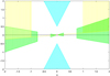 |
Fig. 1 A visual interpretation of conditions (A 1)−(A 4). |
Assumption (A 2) is more difficult to visualize, but the easiest method for finding a function g with this property uses the mean value theorem. Following this method, we can find an easy-to-interpret condition on g that guarantees (A 2) is satisfied. The argument is as follows:
Let g be such that whenever  , g(x) ≠ αx for all
 ![Mathematical equation: $ \alpha \in [m,M]$](/articles/fopen/full_html/2019/01/fopen180047/fopen180047-eq206.gif) . Recall that m and M are the minimum and maximum values of f. This is exactly the contrapositive statement of
. Recall that m and M are the minimum and maximum values of f. This is exactly the contrapositive statement of ![Mathematical equation: $ \exists \alpha \in [m,M]$](/articles/fopen/full_html/2019/01/fopen180047/fopen180047-eq207.gif) such that
such that
 .
.
Now, if  , then the mean value theorem guarantees the existence of a
 ![Mathematical equation: $ \tau \in [\mathrm{0,1}]$](/articles/fopen/full_html/2019/01/fopen180047/fopen180047-eq210.gif) such that
such that  . Obviously,
 ![Mathematical equation: $ f(\tau )\in [m,M]$](/articles/fopen/full_html/2019/01/fopen180047/fopen180047-eq212.gif) , so
, so  , as desired.
This slightly-stronger condition can be represented visually by the green regions in Figure 1. These are for R 1 = 0.25 and R 2 = 0.75, and are formed by plotting the lines y = mx and y = Mx.
We have already made sure that k
1 is such that (A
3) is satisfied. Next, consider (A
4). This condition involves the end behaviour of g as x → ±∞. Let  . If we require that
  for all
  , for some R > 0, then (A
4) will be satisfied. Note, however, that you could also add a vertical shift and require
, for some R > 0, then (A
4) will be satisfied. Note, however, that you could also add a vertical shift and require  for any constant c. We can represent this visually as the yellow regions in Figure 1. If we choose R = 1, then g cannot pass through the yellow region.
The origin in Figure 1 is circled as a reminder that g(0) ≠ 0 in order to have a non-trivial solution.
The equation (1.1) will have a solution for any function g that does not pass through any of the shaded regions. Because of the nature of this image, the functions that might come to mind are those of the form  . However, a (rotated) hyperbolic function also has linear asymptotes. Therefore, another class of functions for which equation (1.1) has a solution would be those of the form
  , where b, c > 0. Obviously, not all values of b and c will keep g in the white regions of Figure 1, but it is easy to find some that do. For example, Figure 2 shows three such choices of b and c, for the parameters we have chosen up until this point.
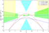 |
Fig. 2 Examples of rotated hyperbolic functions g which satisfy the conditions (A
1)−(A
4). The functions are of the form |

Example 5.2.We can do a similar analysis for Theorem 4.1, and Figure 3 again shows a visual interpretation of some of the conditions for the theorem, with example functions. These examples will conclude with a brief comparison to Theorem 3.1.
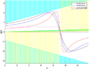 |
Fig. 3 Examples of rational functions |
To understand what types of functions satisfy conditions (B 1)−(B 5), we can first find a function f, and parameters T, R 1, R 2, k 1,and k 2 which are consistent with the conditions. Then, there will be only certain functions g that satisfy all the conditions.
When compared to Theorem 3.1, there is less flexibility in the choices of parameters, due to condition (B 4). If we choose T = 1 and R 1, R 2, k 1, k 2 at random, it is possible to have R > k 1 R 1 + k 2, where,

This would contradict (B
4), because to have  requires that g(x) > R for some
  , but (B
1) requires g(x) < k
1
R
1+k
2 < R in this region. However, one can adjust the parameters until R < k
1
R
1 + k
2.
, but (B
1) requires g(x) < k
1
R
1+k
2 < R in this region. However, one can adjust the parameters until R < k
1
R
1 + k
2.
In the following example, parameters were chosen as follows:
-
T = 1
-
 , so the maximum value of f is 0.02, the minimum value of f is 0.01, and the average value of f is 0.005. Thus,
  .
. -
R 1 = 9, R 2 = 9.25
-
k 1
 0.1722, k
2 = 0.9
0.1722, k
2 = 0.9
Figure 3 shows some examples of functions g that satisfy all the conditions of Theorem 4.1 under these constraints; analysis of the conditions follow.
First, it is easy to check (B 3):
We will consider assumption (B 4) last.
Assumption (B 1) puts the first constraint on g. Represented visually in Figure 3, g(x) cannot pass through the blue regions.
Assumption (B
2) can be handled in the same way as explained in the example for Theorem 3.1. We require g to be such that whenever  , x > 0, we have g(x) ≠ αx for all
 ![Mathematical equation: $ \alpha \in [m,M]$](/articles/fopen/full_html/2019/01/fopen180047/fopen180047-eq228.gif) . Here, m and M are the minimum and maximum values of f. This slightly-stronger condition can be represented visually as the green regions in Figure 3. If we choose R
1 = 9 and R
2 = 9.25, then g cannot pass through these green regions. The green regions are formed by plotting the lines y = mx and y = Mx.
. Here, m and M are the minimum and maximum values of f. This slightly-stronger condition can be represented visually as the green regions in Figure 3. If we choose R
1 = 9 and R
2 = 9.25, then g cannot pass through these green regions. The green regions are formed by plotting the lines y = mx and y = Mx.
Assumption (B
5) is straight-forward to interpret visually. In Figure 3, if g does not pass through the yellow regions, then (B
5) is satisfied. The regions were constructed using the line  , where
  is the average value of f.
When considering (B
4), direct computation of the integral is necessary. However, to help choose a function g with an integral over (0, R
1) greater than R, try to make g stay averaged around a value greater than  ; if g is constant g
0, then we would want g
0⋅R
1 > R.
; if g is constant g
0, then we would want g
0⋅R
1 > R.
The value of R for these parameters is approximately 4.5901, so (B 4) is satisfied.
It is not difficult to find functions with similar behaviour on (0, R
1) but which is unbounded for as x → ∞. For example, multiplying by an appropriately-scaled quadratic in (x − x
0) does the trick, as shown in Figure 4. Here, the functions were multiplied by a quadratic factor of  .
.
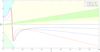 |
Fig. 4 Examples of rational functions |

To compare these examples with those for Theorem 3.1, it is good to notice that there are clearly examples of functions g which satisfy (A 1)−(A 4), but which don’t satisfy (B 5). As an example, Figure 5 shows a visualization of (A 1)−(A 4) for the same parameters and function f as for Figure 4. It is clear that the plotted function satisfies (A 1)−(A 4) but not (B 5), due to the highlighted region. Note that (B 5) only depends on the average value of f and the definition of g, so there is no way to adjust parameters to have (B 5) be satisfied.
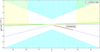 |
Fig. 5 The function |

| a | b |

|
|---|---|---|
| 8 | 4 | 12.315 |
| 2 | 7 | 11.235 |
| 3 | 545 | 7.636 |
6 More examples and simulation
In this section, we see two more examples, with a much more complicated non-linear part. These are also followed by numerical solutions, to further support the results of Theorems 3.1 and 4.1.
Example 6.1.Consider the BVP,

In this example, we have T = 1,  and,
and,

To satisfy (A
1): Let k
1 = 1.5 and k
2 = 100. For,  ,
,

To satisfy (A
2): Let R
1 = 3.5 and R
2 = 200. By direct computation, we know that if g(x) – ϕx = 0 for any constant ![Mathematical equation: $ \phi \in [{\mathrm{min}}_{t\in [\mathrm{0,1}]}f(t),{\mathrm{max}}_{t\in [\mathrm{0,1}]}f(t)]$](/articles/fopen/full_html/2019/01/fopen180047/fopen180047-eq239.gif) , then
, then  .
.
Suppose  . By the mean value theorem, there exists a
 ![Mathematical equation: $ \tau \in [\mathrm{0,1}]$](/articles/fopen/full_html/2019/01/fopen180047/fopen180047-eq242.gif) such that
such that  . Clearly,
 ![Mathematical equation: $ f(\tau )\in [{\mathrm{min}}_{t\in [\mathrm{0,1}]}f(t),{\mathrm{max}}_{t\in [\mathrm{0,1}]}f(t)]$](/articles/fopen/full_html/2019/01/fopen180047/fopen180047-eq244.gif) , so we know that
, so we know that  . Thus, we can conclude that (A
2) is satisfied.
. Thus, we can conclude that (A
2) is satisfied.
To satisfy (A
3): Clearly  and
and

so (A 3) is satisfied.
To satisfy (A
4): We see that  and,
and,

By Theorem 3.1, there exists at least one non-trivial solution for this BVP.
Figure 6 shows a numerical solution obtained by Maple.
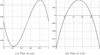 |
Figure 6 Numerical solution for Example 6.1. |
Remark 6.2.For (A
2), the idea is to replace f(t) by a collection of constants ![Mathematical equation: $ {\phi }_t\in [{\mathrm{min}}_{t\in [\mathrm{0,1}]}f(t),{\mathrm{max}}_{t\in [\mathrm{0,1}]}f(t)]$](/articles/fopen/full_html/2019/01/fopen180047/fopen180047-eq250.gif) . We then examine the zeros of g(x)−ϕ
t
x and look for an uniform boundary of all the zeros for all ϕ
t
. By the mean value theorem, such boundary would be the R
1 and R
2 as we desire.
. We then examine the zeros of g(x)−ϕ
t
x and look for an uniform boundary of all the zeros for all ϕ
t
. By the mean value theorem, such boundary would be the R
1 and R
2 as we desire.
Example 6.3.Consider the BVP,
Let T = 1,  and
and
The problem is in the form of equation (1.1).
To satisfy (B 1): Let x > 0, k 1 = 0.001 and k 2 = 0.9905. Then we have,
 and
and

To satisfy (B
2): Let R
1 = 1 and R
1 = 10. By direct computation, we know that if g(x) – ϕx = 0 for any ![Mathematical equation: $ \phi \in [{\mathrm{min}}_{t\in [\mathrm{0,1}]}f(t),{\mathrm{max}}_{t\in [\mathrm{0,1}]}f(t)]$](/articles/fopen/full_html/2019/01/fopen180047/fopen180047-eq256.gif) , then
, then  .
.
Suppose  . By the mean value theorem, there exists a
 ![Mathematical equation: $ \tau \in [\mathrm{0,1}]$](/articles/fopen/full_html/2019/01/fopen180047/fopen180047-eq259.gif) such that
such that  which implies that
  .
.
To satisfy (B 3):

To satisfy (B 4): By computation,

 and
and
Thus, (B 4) is satisfied.
To satisfy (B
5): we calculate that  . For
. For  ,
,

For  ,
,
Thus, (B 5) is satisfied.
By Theorem 4.1, Example 6.3 has at least one positive T-periodic solution. Using Maple, we can find a positive solution for this problem as shown in Figure 7.
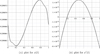 |
Figure 7 Numerical solution for Example 6.3. |
Acknowledgments
The first author was supported by an Undergraduate Student Research Award from NSERC (Natural Sciences and Engineering Research Council of Canada). The third author is supported by a NSERC Discovery Grant.
References
- Zhang L, Wang Y (2010), A note on periodic solutions of a forced Liénard-type equation. Anziam J 51, 350–368. [CrossRef] [Google Scholar]
- Zhang M (1996), Periodic solutions of Liénard equations with singular forces of repulsive type. J Math Anal Appl 203, 254–269. [CrossRef] [Google Scholar]
- Liénard A (1928), Etude des oscillations entretenues. Revue générale de l’électricité 23, 901–912, 946–954. [Google Scholar]
- Tiantian M, Wang Z (2011), Periodic solutions of some second-order differential equations with desultorily sublinear nonlinearities. Nonlinear Anal 74, 41–49. [CrossRef] [Google Scholar]
- Wang Y, Dai X (2009), New results on existence of asymptotically stable periodic solutions of a forced Liénard type equation. Results Math 54, 359–375. [CrossRef] [Google Scholar]
- Zaihong W (2001), Periodic solutions of Liénard differential equations with subquadratic potential conditions. J Math Anal Appl 256, 127–141. [CrossRef] [Google Scholar]
- Wang Z (2002), Existence and multiplicity of periodic solutions of the second order Liénard equation with Lipschtzian condition. Nonlinear Anal 49, 1049–1064. [CrossRef] [Google Scholar]
- Zheng D, Zaihong W (2007), Periodic solutions of sublinear Liénard differential equations. J Math Anal Appl 330, 1478–1487. [CrossRef] [Google Scholar]
- Meng J (2009), Positive periodic solutions for Liénard type p-Laplacian equations. Electron J. Differ. Equ. Paper No. 39, 1–7. [Google Scholar]
- Qiu J (2012), Positive solutions for a nonlinear periodic boundary-value problem with a parameter. Electron J Differ Equ 133, 1–10. [Google Scholar]
- Xin Y, Han X, Cheng Z (2014), Existence and uniqueness of positive periodic solution for Ф-Laplacian Liénard equation. Boundary Value Problems 244, 1–11. [Google Scholar]
- Ding T (1991), On periodic solutions of sublinear duffing equations. J Math Anal Appl 158, 316–332. [CrossRef] [Google Scholar]
- Zamora M (2017), A note on the periodic solutions of a Mathieu-Duffing type equations. Math Nachr 290, 7, 1113–1118. [CrossRef] [Google Scholar]
- Faraday M (1831), On a peculiar class of acoustical figures, and on certain forms assumed by a group of particles upon vibrating elastic surfaces. Philos Trans R Soc Lond Ser B 121, 299–318. [CrossRef] [Google Scholar]
- Natsiavas S, Theodossiades S, Goudas I (2000), Dynamic analysis of piecewise linear oscillators with time periodic coefficients. Int J Non-Linear Mech 35, 53–68. [CrossRef] [Google Scholar]
- Raman A, Bajaj AK, Davies P (1996), On the slow transition across instabilities in non-linear dissipative systems. J Sound Vib 192, 4, 835–865. [CrossRef] [Google Scholar]
- Ye ZM (1997), The non-linear vibration and dynamic instability of thin shallow shells. J Sound Vib 202, 3, 303–311. [CrossRef] [Google Scholar]
- Feng W (2002), Existence for a nonlinear elliptic system at resonance. Dyn Contin Discrete Impuls Syst Ser A Math Anal 9, 69–78. [CrossRef] [Google Scholar]
- Mawhin J (1993), Topological methods for ordinary differential equations. Lect Notes Math 1537, 74–142. [CrossRef] [Google Scholar]
- Feng W, Webb JRL (1997), Solvability of m-point boundary value problems with nonlinear growth. J Math Anal Appl 212, 2, 467–480. [CrossRef] [Google Scholar]
- Feng W (2000), Decomposition conditions for two-point boundary value problems. Int J Math Math Sci 24, 6, 389–401. [CrossRef] [Google Scholar]
- Lu S, Wang Y, Guo Y (2017), Existence of periodic solutions of a Liénard equation with a singularity of repulsive type. Bound Value Probl 95, 1–10. [Google Scholar]
Cite this article as: Korfanty E.R, Liu A & Feng 2019. Periodic solutions for a class of conservative Liénard-type equations. 4open, 2, 5.
All Figures
|
Fig. 1 A visual interpretation of conditions (A 1)−(A 4). |
| In the text | |
|
Fig. 2 Examples of rotated hyperbolic functions g which satisfy the conditions (A
1)−(A
4). The functions are of the form |
| In the text | |
|
Fig. 3 Examples of rational functions |
| In the text | |
|
Fig. 4 Examples of rational functions |
| In the text | |
|
Fig. 5 The function |
| In the text | |
|
Figure 6 Numerical solution for Example 6.1. |
| In the text | |
|
Figure 7 Numerical solution for Example 6.3. |
| In the text | |