© M.T.A. Cordeiro et al., Published by EDP Sciences, 2019

1 Introduction

In the present study, we analyze the entire genome of six autochthonous DENV-1 (Dengue Virus Type 1) strains isolated from patients during the 2014 outbreak in Japan (see [3]). Our objective is to identify the most representative sequence and the least representative sequence of the set. The virus is transmitted to humans by infected mosquitoes of the Aedes genus. The Dengue virus, in their four types, can be contracted more than once, what makes it extremely efficient. Individuals who have already contracted Dengue present risk factors that, by contracting the virus for the second time in a different variant/type, can develop severe forms such as Dengue hemorrhagic fever and Dengue shock syndrome both potentially fatal. In recent years it has been possible to have access to a vaccine, despite this, it is only recommended for those who have already contracted Dengue before. Since the Second World War, the cases of Dengue Fever identified in Japan have been imported, but between 2013 and 2014 more than 160 autochthonous cases were identified. This has demanded a deep investigation of the nature of this outbreak. The contamination has been caused by DENV-1. The findings in [3] suggest that there were at least two independent autochthonous epidemics in Japan in 2014 caused by DENV-1. In this work our objective is to classify the Dengue samples considering the representativeness that each sample has in relation to the group. That is, we know that the samples belong to different individuals and as a consequence are subject to variations in their genomic construction. We wish to identify the most representative sample of the group, this being the most similar to all other samples of the group. Also, we want to identify the most discrepant sample in the group. To achieve our goal, we will identify each sequence with a sample of a stochastic process. Then we will measure the distance between the sequences using a specially designed metric, and applying a robust method (introduced in [1]), we can identify the most representative sample and we can also classify all the samples in order of representativeness. The problem of establishing the proximity between genomic sequences has aroused the interest of several areas and with different objectives. For example, in the area of virology a relevant issue is the characterization of the Epstein Barr virus under different diagnoses, such as Burkitt’s lymphoma, nasopharyngeal carcinoma or even among several types of associated diagnoses [4]. See for examples [5–8], in each case some notion of similarity between strains is explored. An aspect that differentiates this article is that the notion used to establish the proximity between the genomic sequences is a metric (see [2]), that is, it is symmetric, not negative and verifies the triangular inequality. This metric also has very convenient statistical characteristics, such as being statistically consistent. The second aspect and perhaps the most relevant one is the construction of a metric-based classification between the sequences (see [1]). A criterion for classifying samples, statistically consistent as is the case, could be used in the future to construct standard representations for genomic structures. For example, it could certify that the sequence currently used as a gold standard in the Epstein Barr virus study, sequence B95-8, from [9] (see also [5]), in fact, serves impartial criteria such as the one used in this paper.

The sections and topics that compound this article are detailed below. The notions that we use as well as the definition of the criterion to classify the sequences are given in Section 2. We detail the database in Section 3.1. The results are in Section 3.2 and the conclusions in Section 4.

2 Theoretical basis

In this section we give the theoretical framework on which are established, (i) the notion of proximity between sequences as well as (ii) the criterion of classification of the sequences.

Let (X_t) be a discrete time, order o (with o < ∞) Markov chain on a finite alphabet A. Let us call $\mathcal{S}=A^o$ the state space, denote the string a_m, a_m+1,…, a_n by $a_m^n$ where a_i ∈ A, m ≤ i ≤ n. For each a ∈ A and $s\in \mathcal{S}$ define the conditional probability $P\left(a\right|s)= \mathrm{Prob} (X_t=a|X_{t-o}^{t-1}=s).$ In a given sample $x_1^n,$ coming from the stochastic process, the number of occurrences of s in the sample $x_1^n$ is denoted by N_n(s) and the number of occurrences of s followed by a in the sample $x_1^n$ is denoted by N_n(s, a). In this way, $\frac{N_n(s,a)}{N_n\left(s\right)}$ is the estimator of P(a|s). Consider now, two Markov chains (X_1,t) and (X_2,t), of order o, arranged on the finite alphabet A with state space $\mathcal{S}.$ Given $s\in \mathcal{S}$ denote by {P(a|s)}_a∈A and {Q(a|s)}_a∈A the sets of conditional probabilities of (X_1,t) and (X_2,t) respectively. We define a local metric d_s (introduced by [2]) that, when evaluated in a given string s, allows us to define how far or near the processes are.

Definition 2.1. Consider two Markov chains (X_1,t) and (X_2,t), of order o, with finite alphabet A, state space $\mathcal{S}=A^o$ and independent samples $x_{\mathrm{1,1}}^{n_1},$ $x_{\mathrm{2,1}}^{n_2}$ respectively.

1. For a string $s\in \mathcal{S},$

$$d_s(x_{\mathrm{1,1}}^{n_1},x_{\mathrm{2,1}}^{n_2})=\frac{\alpha }{\left(\right|A|-1)\ln (n_1+n_2)}\sum _{a\in A}\mathrm{}\{N_{n_1}(s,a)\ln \left(\frac{N_{n_1}(s,a)}{N_{n_1}\left(s\right)}\right)+N_{n_2}(s,a)\ln \left(\frac{N_{n_2}(s,a)}{N_{n_2}\left(s\right)}\right)-N_{n_1+n_2}(s,a)\ln \left(\frac{N_{n_1+n_2}(s,a)}{N_{n_1+n_2}\left(s\right)}\right)\},$$

$$d_{\max } (x_{\mathrm{1,1}}^{n_1},x_{\mathrm{2,1}}^{n_2})=\underset{s\in \mathcal{S}}{\max }\left\{d_s\right(x_{\mathrm{1,1}}^{n_1},x_{\mathrm{2,1}}^{n_2}\left)\right\},$$ with $N_{n_1+n_2}(s,a)=N_{n_1}(s,a)+N_{n_2}(s,a),$ $N_{n_1+n_2}\left(s\right)=N_{n_1}\left(s\right)+N_{n_2}\left(s\right),$ where $N_{n_1}$ and $N_{n_2}$ are given as usual, computed from the samples $x_{\mathrm{1,1}}^{n_1}$ and $x_{\mathrm{2,1}}^{n_2}$ respectively. With α a real and positive value.

The Definition 2.1 offers us two notions of proximity between sequences, “i.” is local and “ii.” is global, “i.” and “ii.” are statistically consistent, that is, by increasing the min{n₁, n₂} grows their ability to detect (a) discrepancies (when the underlying laws are different) and (b) similarities (when the underlying laws are the same). In the application we use α = 2 (see Definition 2.1-i.), with this value (α = 2), to decide that the sequences follow the same law when d_s < 1, is equivalent to use the Bayesian Information Criterion (see [2, 10]). In [2] is proved also that d_s is a metric:

1. $d_s(x_{\mathrm{1,1}}^{n_1},x_{\mathrm{2,1}}^{n_2})\ge 0 \mathrm{with} \mathrm{equality} \iff \frac{N_{n_1}(s,a)}{N_{n_1}\left(s\right)}=\frac{N_{n_2}(s,a)}{N_{n_2}\left(s\right)} \forall a\in A,$

2. $d_s(x_{\mathrm{1,1}}^{n_1},x_{\mathrm{2,1}}^{n_2})=d_s(x_{\mathrm{2,1}}^{n_2},x_{\mathrm{1,1}}^{n_1}),$

3. $d_s(x_{\mathrm{1,1}}^{n_1},x_{\mathrm{2,1}}^{n_2})\le d_s(x_{\mathrm{1,1}}^{n_1},x_{\mathrm{3,1}}^{n_3})+d_s(x_{\mathrm{3,1}}^{n_3},x_{\mathrm{2,1}}^{n_2}).$

To follow is introduced a notion that makes possible the classification of sequences that belong to a group of sequences.

Definition 2.2. Given a finite collection $\{x_{j,1}^{n_j}{\}}_{j=1}^m$ of samples from the processes $\left\{\right(X_{j,t}){\}}_{j=1}^m$ with probabilities $\{P_j{\}}_{j=1}^m,$ over the finite alphabet A, with state space $\mathcal{S}=A^o$ (o < ∞). For a fixed i ∈ {1, 2,…, m} define

$$V\left(x_{i,1}^{n_i}\right)= \mathrm{median} \left\{d_{\max }\right(x_{i,1}^{n_i},x_{j,1}^{n_j}):j\ne i,1\le j\le m\}.$$ where, given a sequence $\{z_j{\}}_{j=1}^l, \mathrm{median} \{z_j,1\le j\le l\}=z_{(k+1)}$ if l = 2k + 1 and $\mathrm{median} \{z_j,1\le j\le l\}=\frac{z_{\left(k\right)}+z_{(k+1)}}{2}$ if l = 2k, for k an integer and z_(j) denoting the jth order statistic of the collection $\{z_j{\}}_{j=1}^l$.

With the V values attributed to each sample, we can proceed to order the samples, from lowest to highest value of V, in order to identify their classification. As we can perceive from the Definition 2.2, low values of V indicate that these samples represent the whole group better, while high values of V indicate little representativeness. The next result (proved in [1]), give us an adequate tool to classify sequences, according to their underlying laws, it allows to consolidate V as a robust and consistent classifier.

Theorem 2.1. Under the assumptions of Definition 2.2, for each i, 1 ≤ i ≤ m, set ${\xi }_i=\left|\right\{j:1\le j\le m,P_j=P_i\left\}\right|$ ,

$$V\left(x_{i,1}^{n_i}\right)\underset{\min \left\{n_1,\cdots ,n_m\right\}\to \mathrm{\infty }}{\to }\mathrm{\infty }, \mathrm{if}, \mathrm{and} \mathrm{only} \mathrm{if}, \hspace{1em}{\xi }_i\le \lceil \frac{m}{2}\rceil .$$

$$V\left(x_{i,1}^{n_i}\right)\underset{\min \{n_1,\cdots ,n_m\}\to \mathrm{\infty }}{\to }0, \mathrm{if}, \mathrm{and} \mathrm{only} \mathrm{if}, \hspace{1em}{\xi }_i>\lceil \frac{m}{2}\rceil .$$ where $\lceil x\rceil$ is the smallest integer greater than or equal to x. Theorem 2.1 guarantees that if at least 50% of the samples of the set follow the same law, each of them receives a value of V close to zero. And if this does not happen, V takes arbitrarily large values identifying discrepancies in the generating laws of the sequences.

3 Data and results

First, we describe the data, its source and structure, afterwards we proceed to measure the distance between the sequences and to classify them by representativeness.

3.1 Dengue virus type 1

The complete sequences were obtained from http://www.ncbi.nlm.nih.gov/ (NCBI – National Center for Biotechnology Information), sequenced and studied for the first time in [3]. We describe the sequences in Table 1.

The epicenter of Dengue Fever (DF) outbreak during 2014 was possible in the Yoyogi Park in Tokyo. Part of the sequences are coming from patients who pass through there and nearby locations. Details of each patient listed in Table 1 are given in [3], here we emphasize some of them. In the last column of Table 1 we inform the place in where it is suspected that the contamination happened to each patient. The contamination of patient 14-149J occurred in a place near to Yoyogi Park. 14-153J did not visit Yoyogi Park for at least two weeks before the onset of DF and was likely infected in Chiba prefecture. 14-181J lives in Shizuoka prefecture and never visited Yoyogi Park or the other affected areas, visited other places in Tokyo before the onset of DF. Patient 14-188J lives in Nishinomiya city, Hyogo prefecture, over 500 km of Tokyo and never visited the Tokyo area before the onset of DF. He visited Malaysia for seven days and had the onset of DF 12 days after. To illustrate the structure of the data, consider the beginning of the sequence LC011945,

$$\mathrm{gacaagaacagtttcgaatcggaagcttgcttaacgtagttctaacagtt}\dots$$then, the alphabet is A = {a, c, g, t} with cardinal |A| = 4 and elements: adenine (a), cytosine (c), guanine (g) and thymine (t). All the sequences have around a size of 10 700 elements.

In Figure 1 we see a map of Japan with the regions from are coming the patients listed in Table 1. To calculate the classification of the sequences and establish the similarity between them, in the next section we first calculate the values of d_s for each pair of sequences, where s is a state of the state space $\mathcal{S}$. As usual, the elements of the alphabet A are organized in triples, then we can choose a memory o = 3, 6, 9, etc., therefore, the state space is composed of o concatenations of elements of A ($\mathcal{S}=A^o$). In this case, the size of the sequences is approximately 10 700, so the recommended memory is $o<\lfloor {\log }_{\left|A\right|}\left(10700\right)\rfloor -1=7,$ where $\lfloor x\rfloor$ is the greatest integer less than or equal to x. Then we can use memory three or six, to simplify, we use the memory o = 3.

Figure 1 Map of Japan with the regions listed in Table 1.

3.2 Similarity between the genomic sequences

Since we want to obtain global measurements between the sequences we calculate the values of d_max (Definition 2.1-ii.) between each pair of sequences. From this, we found that the three Tokyo sequences, LC011945, LC11946 and LC11947 have d_max = 0. So, the three Tokyo sequences will be represented by LC011945. Then, we will work with four sequences, the sequence names an index number are shown in Table 2. Table 3 shows the value of d_max for each pair of sequences. That is, for each pair of sequences in the Table 2 we compute d_max, the computation of d_max requires the computation of d_s for each s of the state space. And in that case the memory used is o = 3.

We see that the lowest value of d_max is caused by the sequences LC011945 and LC011948, with the second lowest value being the d_max between the sequences LC011945 and LC016760. Already the highest value of d_max occurs between the sequence LC011949 in relation to the sequences LC011945, LC011948 and LC016760 respectively. It is useful to represent the values of d_max through a dendrogram as seen on Figure 2. We build different dendrograms (average, median, single and complete) and they all point to the same organization between the sequences, see http://www.ime.unicamp.br/~jg/cadvj/. As we can see, in fact the dendrogram exposes the homogeneity between three of the four sequences: LC011945, LC011948 and LC016760, leaving exposed the disparity between the sequence LC011949 and the group of three sequences.

Figure 2 Dendrogram by average criterion build from the dmax values, reported in the Table 3.

Observe that d_max < 1 in all cases (Table 3), this implies that all values of d_s < 1 in all states $s\in \mathcal{S},$ i.e. the four sequences are considered as generated by the same stochastic law, but between them exist certain heterogeneity, detected by the magnitudes of d_max. This fact allows us to carry out investigations that answer which of them is more or less representative in the set, which is the approach of the following subsection.

3.3 Classification of each sequence by means of V

We determine the classification attributed to each sequence, according to criterion V (see Definition 2.2). Table 4 shows the results.

The sequence that best represent de set of sequences (listed in Table 2) is coming from Tokyo LC011945. The most discrepant sequence (larger V) is LC011949, being the less representative sample and it indicates that LC011949 may have a different origin than the other sequences. This is, patient 14-181J was probably infected by a different strain from the other Japanese patients of Table 1. Comparing the classification of LC011949, which is 0.04200, we see clearly the impact of the d_max values coming from Table 3. Each time the sequence LC011949 is compared with another one in the list, the value of d_max increases by one decimal.

To identify more strongly the meaning of this classification, we have compared all the sequences found in the base http://www.ncbi.nlm.nih.gov/ with the profile of being complete sequences of Dengue Type 1, year 2014, and coming from Asia. The list of accession numbers is given in the Table 5. For each sequence identified through its accession number we attach two letters to that number, in order to easily identify the country. In Figure 3 we show a dendrogram build by the average criterion with all the complete sequences.

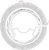Figure 3 Dendrogram by average criterion for the sequences listed in Table 5 build from the dmax values (Definition 2.1-ii.). With arrows we indicate the four Japanese sequences from Table 2.

The circular dendrogram shows that the sequence of Japan (LC011949) with the highest V (among those in the list of Table 4) is in a cluster quite far away from the others in the list (LC011945, LC011948, LC016760). Some observations from Figure 3 can be done, for instance, the Japanese sequence LC011949 is next to the Chinese sequence KT827371, while the other Japanese sequences (Table 4) are closer to a variety of sequences from various countries including Japan, Malaysia and Singapore. Moreover, by the form of organization of the dendrogram, we verified that the sequence LC011949 is considerably more distant from the group {LC011945, LC011948, LC016760} in comparison with other foreign sequences, such as sequences coming from China, Malaysia and Singapore. As seen in Figure 2, the dendrogram of Figure 3 also shows the proximity of the Japanese sequences LC011945 and LC011948, which supports the argument of its representativeness in the group of Table 1. See also http://www.ime.unicamp.br/~jg/cadvj/, in order to corroborate the results with dendrograms build applying several criteria. The Japanese sequence LC011949 (Shizuoka patient who never visited Yoyogi Park) besides being the least representative (V and d_max higher) is also shown in Figure 3 closer to those of Chinese origin, which could implies a contamination of different origin.

4 Conclusion

In this paper we use two stochastic and statistically consistent notions to, (i) establish the proximity between genomic sequences (see [2]), (ii) classify the sequences in terms of their representativeness (see [1]). The classification rule gives low values to more representative sequences and it gives high values to less representative sequences. We classify genomic sequences of Dengue Virus Type I, originating in Japan and all corresponding to the outbreak occurred in Japan during 2014 (see Table 4). We identify the most representative sequences of the outbreak (those are from Tokyo), and we verify that these resemble other sequences (of 2014) coming from countries like Malaysia, Singapore, and China. The less representative sequence of the outbreak (from Shizuoka) is also a sequence that could resemble another one of Chinese origin (from 2014), but the latter being distant from the representative sequences of the outbreak. According to the classification that we have obtained and because of the evidence (see Figs. 2 and 3) we tend to agree with [3] in the sense of affirming that the outbreak in Japan during 2014 could involve more than one type of Dengue Virus Type I. By means of this type of approach it is possible to quantify the representativity of sequences, when compared with groups of sequences. This way of classifying is a genuinely stochastic tool, as explained in Section 2, that reports how close or distant are the stochastic laws of the sequences under consideration.

Future research could include the various serotypes of Dengue virus, in order to, (a) establish whether the notion d_max/d_s is capable of discriminating between the serotypes, (b) identify the spectrum of variation of the classifier (V) in each serotype, (c) establish the impact of the α constant (see Definition 2.1) in (a) and (b).

Acknowledgments

M. Cordeiro and S. Londoño gratefully acknowledge the financial support provided by CAPES with fellowships from the PhD Program in Statistics – University of Campinas. J.E. García and V.A. González-López gratefully acknowledge the support provided by the project Inhibitory deficit as a marker of neuroplasticity in rehabilitation grant 2017/12943-8, São Paulo Research Foundation (FAPESP). Also, the authors wish to thank the three referees for their many helpful comments and suggestions on an earlier draft of this paper.

References

All Tables

All Figures

	Figure 1 Map of Japan with the regions listed in Table 1.
In the text

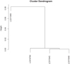	Figure 2 Dendrogram by average criterion build from the dmax values, reported in the Table 3.
In the text

	Figure 3 Dendrogram by average criterion for the sequences listed in Table 5 build from the dmax values (Definition 2.1-ii.). With arrows we indicate the four Japanese sequences from Table 2.
In the text

References

- Fernández M, García Jesús E, Gholizadeh R, González-López VA (2019), Sample selection procedure in daily trading volume processes. Math Meth Appl Sci, 1–13. https://doi.org/10.1002/mma.5705. [Google Scholar]
- García Jesús E, Gholizadeh R, González-López VA (2018), A BIC-based consistent metric between Markovian processes. Appl Stoch Models Bus Ind 34, 6, 868–878. [Google Scholar]
- Tajima S, Nakayama E, Kotaki A, Moi ML, Ikeda M, Yagasaki K, Saito Y, Shibasaki K, Saijo M, Takasaki T (2017), Whole genome sequencing–based molecular epidemiologic analysis of autochthonous dengue virus type 1 strains circulating in Japan in 2014. Jpn J infect Dis 70, 1, 45–49. [CrossRef] [PubMed] [Google Scholar]
- Liu P, Fang X, Feng Z, Guo YM, Peng RJ, Liu T, Huang Z, Feng Y, Sun X, Xiong Z, Guo X, Pang SS, Wang B, Lv X, Feng FT, Li DJ, Chen LZ, Feng QS, Huang WL, Zeng MS, Bei JX, Zhang Y, Zeng YX (2011), Direct sequencing and characterization of a clinical isolate of Epstein-Barr virus from nasopharyngeal carcinoma tissue by using next-generation sequencing technology. J Virol 85, 21, 11291–11299. [CrossRef] [PubMed] [Google Scholar]
- Zeng MS, Li DJ, Liu QL, Song LB, Li MZ, Zhang RH, Yu XJ, Wang HM, Emberg I, Zeng YX (2005), Genomic sequence analysis of Epstein-Barr Virus strain GD1 from a nasopharyngeal carcinoma patient. J Virol 79, 24, 15323–15330. [CrossRef] [PubMed] [Google Scholar]
- Kwok H, Tong AH, Lin CH, Lok S, Farrel PJ, Kwong DL, Chiang AK (2012), Genomic sequencing and comparative analysis of Epstein-Barr Virus genome isolated from primary nasopharyngeal carcinoma biopsy. PLoS One 7, 5, e36939. [CrossRef] [PubMed] [Google Scholar]
- García Jesús E, González-López VA (2016), Markov partition models for Epstein Barr virus, in: JR Bozeman Jr, T Oliveira, CH Skiadas (Eds.), Stochastic and Data Analysis Methods and Applications in Statistics and Demography, International Society for the Advancement of Science and Technology (ISAST), Athens. [Google Scholar]
- García Jesús E, Gholizadeh R, González-López VA (2018), Stochastic distance between Burkitt lymphoma/leukemia strains, in: C Skiadas, C Skiadas (Eds.), Demography and Health Issues. The Springer Series on Demographic Methods and Population Analysis, Vol. 46, Springer, Cham. [Google Scholar]
- Baer R, Bankier AT, Biggin MD, Deininger PL, Farrell PJ, Gibson TJ, Hatfull G, Hudson GS, Satchwell SC, Seguin C, Tuffnell PS, Barrell BG (1984), DNA sequence and expression of the B95–8 Epstein-Barr virus genome. Nature 310, 5974, 207. [CrossRef] [PubMed] [Google Scholar]
- Schwarz G (1978), Estimating the dimension of a model. Ann Stat 6, 2, 461–464. [Google Scholar]
Cite this article as: Cordeiro MTA, García JE, González-López VA & Londoño SLM 2019. Classification of autochthonous dengue virus type 1 strains circulating in Japan in 2014. 4open, 2, 20.
All Tables
Complete Sequences of Dengue Virus Type 1. Columns from left to right: (1) the identification of the sequence/strain, (2) the number of access to the NCBI base, (3) the patient from which it is coming the sequence, (4) the possible local of contamination of the patient.
List of accession numbers (NCBI base) of complete sequences of Dengue virus Type 1, year 2014 – from Asia. The first column shows the country and the second column shows the sequences coming from the country, on the left.