© P.E. Ricci, Published by EDP Sciences, 2020

Introduction

In preceding articles, starting from Bernoulli’s spiral, in the complex form, we have highlithed the obvious connection between the first and second kind Chebyshev polynomials, and the Grandi (Rodhonea) curves.

As these curves exist even for rational index values, we have extended these Chebyshev polynomials to the case of fractional degree [1]. The resulting functions are no more polynomials, but irrational functions that have been called pseudo-Chebyshev functions, because they satisfy many properties of the corresponding Chebyshev polynomials. Actually the irrationality of these functions is due to a constant factor which is multiplied by polynomials.

In subsequent articles [2, 3], recalling the third and fourth kind Chebyshev polynomials, and their connections to the preceding ones, as it is presented in [4], we have also introduced, for completeness, the corresponding pseudo-Chebyshev functions of the third and fourth kind. It has been shown that these families of functions satisfy the recursion and differential equations of the classical Chebyshev polynomials up to the change of the degree (from the integer to the fractional one). The particular case which seems to be the most important one, is when the degree is of the type k + 1/2, that is a half-integer, since in this case, the pseudo-Chebyshev functions satisfy even the orthogonality properties, in the interval (−1, 1), with respect to the same weights of the classical polynomials.

Archimedes vs. Bernoulli spiral

Spirals are described by polar equations and, in a recent work [1], has been highlithed the connection of the Bernoulli spiral, in complex form, with the Grandi (Rhodonea) curves and the Chebyshev polynomials.

The Archimedes spiral [5] (Fig. 1) has the polar equation:$$\begin{array}{l}\rho =a \theta ,\hspace{1em} (a>0,\hspace{0.5em}\theta \in {\mathbb{R}}^{+}).\end{array}$$(1)

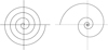Figure 1 Archimedes vs. Bernoulli spiral.

If θ > 0 the spiral turns counter-clockwise, if θ < 0 the spiral turns clockwise. Bernoulli’s (logarithmic) spiral [6] (Fig. 1) has the polar equation$$\begin{array}{l}\rho =a b^{\theta }, \hspace{1em}(a,b\in {\mathbb{R}}^{+}), \hspace{1em}\theta ={\log }_b\left(\rho /a\right).\end{array}$$(2)

By changing the parameters a and b one gets different types of spirals.

The size of the spiral is determined by a, while the verse of rotation and how it is “narrow” depend on b.

Being a and b positive costants, there are some interesting cases. The most popular logarithmic spiral is the harmonic spiral, also called Fibonacci spiral, in which the distance between the spires is in harmonic progression, with ratio $\varphi =\frac{\sqrt{5}-1}{2}$, that is, the “Golden ratio”.

The logarithmic spiral was discovered by René Descartes in 1638, and studied by Jakob Bernoulli (1654–1705).

It is a first example of a fractal. On J. Bernoulli’s tomb there is the sentence: Eadem Mutata Resurgo.

In what follows, we consider a “canonical form” of the Bernoulli spirals assuming a = 1, b = eⁿ, that is the simplified polar equation:$$\rho =e^{n \theta }, \hspace{1em}(n\in N).$$(3)

The complex Bernoulli spiral

In the complex case, putting$$\begin{array}{l}\rho =\mathfrak{R}\rho +\mathrm{i} \mathfrak{I}\rho ,\end{array}$$(4)and considering the Bernoulli spiral:$$\begin{array}{l}\rho =e^{\mathrm{i} \mathrm{n\theta }}=\cos \mathrm{n\theta }+\mathrm{i} \sin \mathrm{n\theta },\end{array}$$(5)we find:$$\begin{array}{l}{\rho }_1=\mathfrak{R}\rho =\cos \mathrm{n\theta }, \hspace{1em}{\rho }_2=\mathfrak{I}\rho =\sin \mathrm{n\theta }.\end{array}$$(6)

Recalling Chebyshev polynomials

Starting from the equations:$$(e^{\mathrm{i} t}{)}^n=e^{\mathrm{i} \mathrm{nt}}, (\cos t+\mathrm{i} \sin t{)}^n=\cos \left(\mathrm{nt}\right)+\mathrm{i} \sin \left(\mathrm{nt}\right),$$(7)separating the real from the imaginary part, and putting x = cos t, the first and second kind Chebyshev polynomials are derived:$$T_n\left(x\right) ≔\cos (n \arccos x)=\sum _{h=0}^{\left[\frac{n}{2}\right]}\mathrm{}(-1{)}^h\left(\begin{array}{c}n\\ 2h\end{array}\right)x^{n-2h}(1-x^2{)}^h,$$(8)$$U_{n-1}\left(x\right) ≔\frac{\sin (n \arccos x)}{\sin \left(\arccos x\right)}=\sum _{h=0}^{\left[\frac{n-1}{2}\right]}\mathrm{} (-1{)}^h\left(\begin{array}{c}n\\ 2h+1\end{array}\right)x^{n-2h-1}(1-x^2{)}^h.$$(9)

It is well known that the first kind Chebyshev polynomials [7] play an important role in Approximation theory, since their zeros constitute the nodes of optimal interpolation, because their choice minimizes the error of interpolation. They’re also the optimal nodes for the Gaussian quadrature rules.

The second kind Chebyshev polynomials can be used for representing the powers of a 2 × 2 non singular matrix [8]. Extension of this polynomial falmily to the multivariate case has been considered for the powers of a r × r (r ≥ 3) non singular matrix (see [9, 10]).

Remark 1

Chebyshev polynomials are a particular case of the Jacobi polynomials $P_n^{(\alpha ,\beta )}\left(x\right)$ [11], which are orthogonal in the interval [−1, 1] with respect to the weight $(1-x{)}^{\alpha }(1+x{)}^{\beta }$. More precisely, the following equations hold:$$T_n\left(x\right)=P_n^{(-1/2,-1/2)}\left(x\right), \hspace{1em}{U}_n\left(x\right)=P_n^{(1/\mathrm{2,1}/2)}\left(x\right).$$Therefore, properties of the Chebyshev polynomials could be deduced in the framework of hypergeometric functions. However, in this more general approach, the connection with trigonomeric functions disappears.

Remark 2

In connection with interpolation and quadrature problems, two other types of Chebyshev polynomials have been considered. They correspond to different choices of weights:$$V_n\left(x\right)=P_n^{(1/2,-1/2)}\left(x\right), \hspace{1em}{W}_n\left(x\right)=P_n^{(-1/\mathrm{2,1}/2)}\left(x\right).$$

These were called by Gautschi [12] the third and fourth kind Chebyshev polynomials, and have been used in Numerical Analysis, mainly in the framework of quadrature rules.

Basic properties of the Chebyshev polynomials of third and fourth kind

The third and fourth kind Chebyshev polynomials have been used by many scholars (see e.g. [4, 13]), because they are useful in particular quadrature rules, when singularities of the integrating function occur only at one end of the considered interval, that is (+1 or −1) (see [14, 15]). They have been shown even to be useful for solving high odd-order boundary value problems with homogeneous or nonhomogeneous boundary conditions [13].

The third and fourth kind Chebyshev polynomials are defined in $[-\mathrm{1,1}]$ as follows:$$\begin{array}{l}{V}_n\left(x\right)=\frac{\cos \left[(n+1/2)\arccos x\right]}{\cos \left[\right(\arccos x)/2]},\\ W_n\left(x\right)=\frac{\sin \left[(n+1/2)\arccos x\right]}{\sin \left[\right(\arccos x)/2]}.\end{array}$$(10)

Since $W_n\left(x\right)=(-1{)}^n{V}_n(-x)$, as it can be see by their graphs (Figs. 2 and 3), the third and fourth kind Chebyshev polynomials are essentially the same polynomial set, but interchanging the ends of the interval $[-\mathrm{1,1}]$.

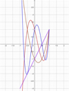Figure 2 Vk (x), k = 1, 2, 3, 4. (1) Violet; (2) brown; (3) red; (4) blue.

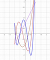Figure 3 Wk (x), k = 1, 2, 3, 4. (1) Violet; (2) brown; (3) red; (4) blue.

The orthogonality properties hold [4]:$${\int }_{-1}^1\mathrm{}{V}_n\left(x\right)V_m\left(x\right) \sqrt{\frac{1+x}{1-x}} \mathrm{d}x={\int }_{-1}^1\mathrm{}{W}_n\left(x\right)W_m\left(x\right) \sqrt{\frac{1-x}{1+x}} \mathrm{d}x=\pi {\delta }_{n,m},$$(δ is the Kronecher delta).

One of the explicit advantages of Chebyshev polynomials of third and fourth kind is to estimate some definite integrals as$${\int }_{-1}^1\mathrm{}\sqrt{\frac{1+x}{1-x}} f\left(x\right)\mathrm{d}x\hspace{1em}\mathrm{and}\hspace{1em}{\int }_{-1}^1\mathrm{}\sqrt{\frac{1-x}{1+x}} f\left(x\right) \mathrm{d}x$$with the precision degree 2n − 1, by using the n interpolatory points $x_k=\cos \frac{(2k-1)\pi }{2n+1}$, (k = 1, 2, …, n), in the interval [−1, 1] [13, 14].

The Grandi (Rhodonea) curves

The curves with polar equation:$$\rho =\cos \left(\mathrm{n\theta }\right)$$(11)are known as Rhodonea or Grandi curves, in honour of G. Guido Grandi who communicated his discovery to G.W. Leibniz in 1713.

Curves with polar equation: $\rho =\sin \left(\mathrm{n\theta }\right)$ are equivalent to the preceding ones, up to a rotation of $\pi /\left(2n\right)$ radians.

The Grandi roses display

• n petals, if $n$ is odd,

• 2n petals, if $n$ is even.

By using equation (11) it is impossible to obtain, roses with $4n+2$($n\in N\cup \left\{0\right\}$) petals.

Roses with $4n+2$ petals can be obtained by using the Bernoulli Lemniscate and its extensions. More precisely,

• for n = 0, a two petals rose comes from the equation $\rho ={\cos }^{1/2}\left(2\theta \right),$ (the Bernoulli Lemniscate),

• for n ≥ 1, a 4n + 2 petals rose comes from the equation $\rho ={\cos }^{1/2}\left[\right(4n+2\left)\theta \right]$.

A few graphs of Rhodonea curves are shown in Figures 4–7.

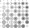Figure 4 Rhodonea $\cos \left(\frac{p}{q} \theta \right).$

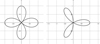Figure 5 Rhodonea cos(2θ) and cos(3θ).

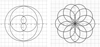Figure 6 Rodoneas $\cos \left(\frac{1}{4} \theta \right)$ and $\cos \left(\frac{5}{4} \theta \right)$.

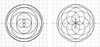Figure 7 Rodoneas $\cos \left(\frac{1}{8} \theta \right)$ and $\cos \left(\frac{3}{8} \theta \right)$.

Pseudo-Chebyshev functions of half-integer degree

In what follows, we consider the case of the half-integer degree, which seems to be the most interesting one, since the resulting pseudo-Chebyshev functions satisfy the orthogonality properties in the interval (−1, 1) with respect to the same weights of the corresponding Chebyshev polynomials.

Definition 1

Let, for any integer $k$:$$\begin{array}{l}{T}_{k+\frac{1}{2}}\left(x\right)=\cos \left(\left(k+\frac{1}{2}\right) \arccos \left(x\right)\right),\\ \sqrt{1-x^2} U_{k-\frac{1}{2}}\left(x\right)=\sin \left(\left(k+\frac{1}{2}\right) \arccos \left(x\right)\right),\\ \sqrt{1-x^2} V_{k+\frac{1}{2}}\left(x\right)=\cos \left(\left(k+\frac{1}{2}\right) \arccos \left(x\right)\right),\\ W_{k+\frac{1}{2}}\left(x\right)=\sin \left(\left(k+\frac{1}{2}\right) \arccos \left(x\right)\right).\end{array}$$(12)

Note that the above definition holds even for k + 1/2 < 0, taking into account the parity properties of the circular functions.

Recursion for the $T_{k+\frac{1}{2}}\left(x\right)$ and $W_{k+\frac{1}{2}}\left(x\right)$

Put for shortness: $y_k≔T_{k+\frac{1}{2}}$ and ${\phi }_k≔W_{k+\frac{1}{2}}$. Then, by using definition (12) and the addition formulas for the sine and cosine functions we find:$$\begin{array}{c}{y}_{k+2}= {\mathrm{xy}}_{k+1}+\sqrt{1-x^2} {\phi }_{k+1},\\ {\phi }_{k+2}=x {\phi }_{k+1}-\sqrt{1-x^2} y_{k+1},\end{array}$$and therefore:$$\begin{array}{l}{y}_{k+2}=x{y}_{k+1}+\sqrt{1-x^2} (x {\phi }_k-\sqrt{1-x^2} y_k)=\\ x{y}_{k+1}+x (\sqrt{1-x^2} {\phi }_k+x{y}_k)-y_k=2x{y}_{k+1}-y_k,\end{array}$$that is the same recursion of the classical Chebyshev polynomials:$$\begin{array}{l}{y}_{k+2}=2x y_{k+1}-y_k.\end{array}$$(13)

Furthermore, the initial conditions for the $T_{k+\frac{1}{2}}\left(x\right)$ functions are:$$T_{\pm \frac{1}{2}}\left(x\right)=\sqrt{\frac{1+x}{2}}.$$(14)

Interchanging the roles of $y_k$ and ${\phi }_k$ we find that the same recurrence for second sequence holds, but with different initial conditions. We have, precisely:$$W_{\pm \frac{1}{2}}\left(x\right)=\pm \sqrt{\frac{1-x}{2}}.$$(15)

Differential equations for the $T_{k+\frac{1}{2}}\left(x\right)$ and $W_{k+\frac{1}{2}}\left(x\right)$

Even the differential equations satified by the $y_k$ and ${\phi }_k$ can be recovered by using a coupled technique. In fact, differentating $y_k$ and ${\phi }_k$, we find:$$\sqrt{1-x^2} y_k^{\prime }-(k+1/2){\phi }_k=0,$$$$\sqrt{1-x^2} {\phi }_k^{\prime }+(k+1/2)y_k=0,$$and differentiating again the first equation:$${\sqrt{1-x^2} y_k^{″}-\frac{x}{\sqrt{1-x^2}} \mathrm{y\text{'}}}_k-(k+1/2){\phi \prime }_k=0,$$that is:$${(1-x^2)y_k^{″}-x y_k^{\prime }-\sqrt{1-x^2} (k+1/2)\phi \prime }_k=0.$$

Substituting ${\phi \prime }_k$, we find the differential equation satisfied by the $y_k$:$$(1-x^2)y_k^{″}-x y_k^{\prime }+{\left(k+\frac{1}{2}\right)}^2{y}_k=0.$$(16)and interchanging the roles of $y_k$ and ${\phi }_k$ we find that the same differential equation is satisfied by the ${\phi }_k$.

Remark 3

The first few $T_{k+\frac{1}{2}}\left(x\right)$ are:$$\begin{array}{l}{T}_{\frac{1}{2}}\left(x\right)=\sqrt{\frac{1+x}{2}}\\ T_{\frac{3}{2}}\left(x\right)=\sqrt{\frac{1+x}{2}} (2x-1)\\ T_{\frac{5}{2}}\left(x\right)=\sqrt{\frac{1+x}{2}} (4x^2-2x-1)\\ T_{\frac{7}{2}}\left(x\right)=\sqrt{\frac{1+x}{2}} (8x^3-4x^2-4x+1)\\ T_{\frac{9}{2}}\left(x\right)=\sqrt{\frac{1+x}{2}} (16x^4-8x^3-12x^2+4x+1)\end{array}$$

Remark 4

The first few $W_{k+\frac{1}{2}}\left(x\right)$ are:$$\begin{array}{l}{W}_{\frac{1}{2}}\left(x\right)=\sqrt{\frac{1-x}{2}}\\ W_{\frac{3}{2}}\left(x\right)=\sqrt{\frac{1-x}{2}} (2x+1)\\ W_{\frac{5}{2}}\left(x\right)=\sqrt{\frac{1-x}{2}} (4x^2+2x-1)\\ W_{\frac{7}{2}}\left(x\right)=\sqrt{\frac{1-x}{2}} (8x^3+4x^2-4x-1)\\ W_{\frac{9}{2}}\left(x\right)=\sqrt{\frac{1-x}{2}} (16x^4+8x^3-12x^2-4x+1)\end{array}$$

The case of the $U_{k-\frac{1}{2}}\left(x\right)$ and $V_{k+\frac{1}{2}}\left(x\right)$

Recalling equation (12), since$$U_{k-\frac{1}{2}}\left(x\right)=(1-x^2{)}^{-1/2}{\mathrm{W}}_{k+\frac{1}{2}}(x)$$and$$V_{k+\frac{1}{2}}\left(x\right)=(1-x^2{)}^{-1/2}{T}_{k+\frac{1}{2}}(x)$$it results that the functions $U_{k-\frac{1}{2}}\left(x\right)$ and $V_{k+\frac{1}{2}}\left(x\right)$ satisfy the same recursion (13) of the classical Chebyshev polynomials, but with the initial conditions:$$U_{-\frac{3}{2}}\left(x\right)=-\sqrt{\frac{1}{2(1+x)}}, {\hspace{1em}U}_{-\frac{1}{2}}\left(x\right)=\sqrt{\frac{1}{2(1+x)}},$$(17)and$$V_{\pm \frac{1}{2}}\left(x\right)=\sqrt{\frac{1}{2(1-x)}}.$$(18)

Differential equations for the $U_{k-\frac{1}{2}}\left(x\right)$ and $V_{k+\frac{1}{2}}\left(x\right)$

Put for shortness: $z_k≔U_{k-\frac{1}{2}}$ and ${\psi }_k≔V_{k+\frac{1}{2}}$. Differentiating the second equation (12), we find:$$-\frac{x}{\sqrt{1-x^2}} z_k+\sqrt{1-x^2} z_k^{\prime }=-(k+1/2) \frac{1}{\sqrt{1-x^2}} \cos \left(\left(k+\frac{1}{2}\right) \arccos \left(x\right)\right),$$that is$$-x z_k+(1-x^2) z_k^{\prime }+ (k+1/2)\cos \left(\left(k+\frac{1}{2}\right) \arccos \left(x\right)\right)=0,$$and differentiating again, it results:$$-z_k-3x z_k^{\prime }+(1-x^2) {\mathrm{z\text{'}\text{'}}}_k+-(k+1/2{)}^2{z}_k=0,$$that is$${\begin{array}{ll}(1-x^2) z_k^{″}& \end{array}-3x \mathrm{z\text{'}}}_k+\left[{\left(k+\frac{1}{2}\right)}^2-1\right] z_k=0.$$(19)and interchanging the roles of $z_k$ and ${\psi }_k$ we find that the same differential equation is satisfied by the ${\psi }_k$.

Remark 5

The first few $U_{k-\frac{1}{2}}\left(x\right)$ are:$$\begin{array}{l}{U}_{\frac{1}{2}}\left(x\right)=\sqrt{\frac{1}{2(1+x)}} (2x+1)\\ U_{\frac{3}{2}}\left(x\right)=\sqrt{\frac{1}{2(1+x)}} (4x^2+2x-1)\\ U_{\frac{5}{2}}\left(x\right)=\sqrt{\frac{1}{2(1+x)}} (8x^3+4x^2-4x-1)\\ U_{\frac{7}{2}}\left(x\right)=\sqrt{\frac{1}{2(1+x)}} (16x^4+8x^3-12x^2-4x+1)\\ U_{\frac{9}{2}}\left(x\right)=\sqrt{\frac{1}{2(1+x)}} (32x^5+16x^4-32x^3-12x^2+6x+1)\end{array}$$and, in general:$$\sqrt{2(1+x)} U_{k-\frac{1}{2}}\left(x\right)=\sqrt{\frac{2}{1-x}} W_{k+\frac{1}{2}}\left(x\right)$$

Remark 6

The first few $V_{k+\frac{1}{2}}\left(x\right)$ are:$$\begin{array}{l}{V}_{\frac{1}{2}}\left(x\right)=\sqrt{\frac{1}{2(1-x)}}\\ V_{\frac{3}{2}}\left(x\right)=\sqrt{\frac{1}{2(1-x)}} (2x-1)\\ V_{\frac{5}{2}}\left(x\right)=\sqrt{\frac{1}{2(1-x)}} (4x^2-2x-1)\\ V_{\frac{7}{2}}\left(x\right)=\sqrt{\frac{1}{2(1-x)}} (8x^3-4x^2-4x+1)\\ V_{\frac{9}{2}}\left(x\right)=\sqrt{\frac{1}{2(1-x)}} (16x^4-8x^3-12x^2+4x+1)\end{array}$$and, in general:$$\sqrt{2(1-x)} V_{k+\frac{1}{2}}\left(x\right)=\sqrt{\frac{2}{1+x}} T_{k+\frac{1}{2}}\left(x\right)$$

The pseudo-Chebyshev functions $T_{k+\frac{1}{2}}\left(x\right)$, $U_{k-\frac{1}{2}}\left(x\right)$, $V_{k+\frac{1}{2}}\left(x\right)$ and $W_{k+\frac{1}{2}}\left(x\right)$ can be represented, in terms of the third and fourth kind Chebyshev polynomials as follows:$$\begin{array}{l}{T}_{k+\frac{1}{2}}\left(x\right)=\sqrt{\frac{1+x}{2}} V_k\left(x\right),\\ \sqrt{1-x^2} U_{k-\frac{1}{2}}\left(x\right)=\sqrt{\frac{1}{2(1+x)}} W_k\left(x\right),\\ \sqrt{1-x^2} V_{k+\frac{1}{2}}\left(x\right)=\sqrt{\frac{1}{2(1-x)}} V_k\left(x\right),\\ W_{k+\frac{1}{2}}\left(x\right)=\sqrt{\frac{1-x}{2}} W_k\left(x\right).\end{array}$$(20)

In the considered case of half-integer degree, the pseudo-Chebyshev functions satisfy not only the recurrence relations and differential equations analogues to the classical ones, but even the orthogonality properties.

Orthogonality properties of the $T_{k+1/2}\left(x\right)$and $U_{k+1/2}\left(x\right)$functions

A few graphs of the $T_{k+\frac{1}{2}}$ functions are shown in Figure 8.

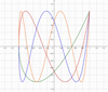Figure 8 Tk+1/2(x), k = 1, 2, 3, 4. (1) Green; (2) red; (3) blue; (4) orange.

Theorem 1

The pseudo-Chebyshev functions $T_{k+1/2}\left(x\right)$satisfy the orthogonality property:$$\begin{array}{l}{\int }_{-1}^1\mathrm{}{T}_{h+\frac{1}{2}}\left(x\right) T_{k+\frac{1}{2}}\left(x\right)\frac{1}{\sqrt{1-x^2}} \mathrm{dx}=0,\hspace{1em} (h\ne k),\end{array}$$(21)where $h,k \mathrm{are} \mathrm{integer} \mathrm{numbers},$$${\int }_{-1}^1\mathrm{}{T}_{k+\frac{1}{2}}^2\left(x\right)\frac{1}{\sqrt{1-x^2}} \mathrm{dx}=\frac{\pi }{2}.$$(22)

A few graphs of the $U_{k+\frac{1}{2}}$ functions are shown in Figure 9.

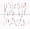Figure 9 Uk+1/2(x), k = 1, 2, 3, 4. (1) Green; (2) red; (3) blue; (4) orange.

Theorem 2

The pseudo-Chebyshev functions $U_{k+\frac{1}{2}}\left(x\right)$ satisfy the orthogonality property:$$\begin{array}{l}{\int }_{-1}^1\mathrm{}{U}_{h+\frac{1}{2}}\left(x\right) U_{k+\frac{1}{2}}\left(x\right)\sqrt{1-x^2} \mathrm{dx}=0,\hspace{1em} (m\ne n),\end{array}$$(23)where $h,k \mathrm{are} \mathrm{integer} \mathrm{numbers},$$${\int }_{-1}^1\mathrm{}{U}_{k+\frac{1}{2}}^2\left(x\right) \sqrt{1-x^2} \mathrm{dx}=\frac{\pi }{2}.$$(24)

Proof. We prove only Theorem 12, since the proof of Theorem 13 is similar.

From the Werner formulas, we have:$$\begin{array}{l}{\int }_{-1}^1\mathrm{}\cos \left[\left(h+\frac{1}{2}\right)\arccos \left(x\right)\right] \cos \left[\left(k+\frac{1}{2}\right)\arccos \left(x\right)\right]\frac{1}{\sqrt{1-x^2}} \mathrm{d}x=\\ \end{array}2 {\int }_0^{\pi /2}\mathrm{}\cos \left[\right(2h+1\left)t\right]\cos \left[\right(2k+1\left)t\right] \mathrm{d}t=0,$$and$$\begin{array}{l}{\int }_{-1}^1\mathrm{}{\cos }^2\left[\left(k+\frac{1}{2}\right)\arccos \left(x\right)\right]\frac{1}{\sqrt{1-x^2}} \mathrm{dx}= 2 {\int }_0^{\frac{\pi }{2}}\mathrm{}{\cos }^2\left(\left(2k+1\right)t\right)\mathrm{d}t=\frac{\pi }{2}.\end{array}$$□

The third and fourth kind pseudo-Chebyshev functions

The results of this section are based on the excellent survey by Aghigh et al. [4]. By using that article, it is possible to derive, in an almost trivial way, the links among the pseudo-Chebyshev functions and the third and fourth kind Chebyshev polynomials.

We recall here only the principal properties, without proofs. Proofs and other properties are reported in reference [3]. In Figures 10 and 11, we show the graphs of the first few third and fourth kind pseudo-Chebyshev functions.

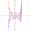Figure 10 Vk+1/2(x), k = 1, 2, 3, 4, 5. (1) Grey; (2) red; (3) blue; (4) orange; (5) violet.

Figure 11 Wk+1/2(x), k = 1, 2, 3, 4, 5. (1) Red; (2) blue; (3) orange; (4) violet; (5) grey.

Orthogonality properties of the $V_{k+1/2}\left(x\right)$and $W_{k+1/2}\left(x\right)$functions

A few graphs of the $V_{k+\frac{1}{2}}$ functions are shown in Figure 10.

Theorem 3

The pseudo-Chebyshev functions $V_{k+1/2}\left(x\right)$verify the orthogonality property:$$\begin{array}{l}{\int }_{-1}^1\mathrm{}{V}_{h+\frac{1}{2}}\left(x\right) V_{k+\frac{1}{2}}\left(x\right) \sqrt{1-x^2} \mathrm{dx}=0, \hspace{1em}(h\ne k),\end{array}$$(25)$${\int }_{-1}^1\mathrm{}{V}_{k+\frac{1}{2}}^2\left(x\right) \sqrt{1-x^2} \mathrm{dx}=\frac{\pi }{2}.$$(26)

A few graphs of the $W_{k+\frac{1}{2}}$ functions are shown in Figure 11.

Theorem 4

The pseudo-Chebyshev functions $W_{k+1/2}\left(x\right)$verify the orthogonality property:$$\begin{array}{l}{\int }_{-1}^1\mathrm{}{W}_{h+\frac{1}{2}}\left(x\right) W_{k+\frac{1}{2}}\left(x\right) \frac{1}{\sqrt{1-x^2}} \mathrm{dx}=0,\hspace{1em} (h\ne k),\end{array}$$(27)$${\int }_{-1}^1\mathrm{}{W}_{k+\frac{1}{2}}^2\left(x\right) \frac{1}{\sqrt{1-x^2}} \mathrm{dx}=\frac{\pi }{2}.$$(28)

Explicit forms

Theorem 5

It is possible to represent explicitly the pseudo-Chebyshev functions as follows: $$\begin{array}{l}{T}_{k+\frac{1}{2}}\left(x\right)=\sqrt{\frac{1+x}{2}} \sum _{h=0}^k\mathrm{}(-1{)}^h\left(\begin{array}{c}2k+1\\ 2h\end{array}\right){\left(\frac{1-x}{2}\right)}^h{\left(\frac{1+x}{2}\right)}^{k-h},\\ U_{k-\frac{1}{2}}\left(x\right)=\sqrt{\frac{1}{2(1+x)}} \sum _{h=0}^k\mathrm{}(-1{)}^h\left(\begin{array}{c}2k+1\\ 2h+1\end{array}\right){\left(\frac{1-x}{2}\right)}^h{\left(\frac{1+x}{2}\right)}^{k-h},\\ V_{k+\frac{1}{2}}\left(x\right)=\sqrt{\frac{1}{2(1-x)}} \sum _{h=0}^k\mathrm{}(-1{)}^h\left(\begin{array}{c}2k+1\\ 2h\end{array}\right){\left(\frac{1-x}{2}\right)}^h{\left(\frac{1+x}{2}\right)}^{k-h},\\ W_{k+\frac{1}{2}}\left(x\right)=\sqrt{\frac{1-x}{2}} \sum _{h=0}^k\mathrm{}(-1{)}^h\left(\begin{array}{c}2k+1\\ 2h+1\end{array}\right){\left(\frac{1-x}{2}\right)}^h{\left(\frac{1+x}{2}\right)}^{k-h}.\end{array}$$(29)

Location of zeros

By equation (12), the zeros of the pseudo-Chebyshev functions $T_{k+\frac{1}{2}}\left(x\right)$ and $V_{k+\frac{1}{2}}\left(x\right)$ are given by$$\begin{array}{l}{x}_{k,h}=\cos \left(\frac{(2h-1)\pi }{2k+1}\right), \hspace{1em}(h=\mathrm{1,2},\dots ,k),\end{array}$$(30)and the zeros of the pseudo-Chebyshev functions $U_{k+\frac{1}{2}}\left(x\right)$ and $W_{k+\frac{1}{2}}\left(x\right)$ are given by$$\begin{array}{l}{x}_{k,h}=\cos \left(\frac{2\mathrm{h\pi }}{2k+1}\right), \hspace{1em}(h=\mathrm{1,2},\dots ,k),\end{array}$$(31)furthermore, the $W_{k+\frac{1}{2}}\left(x\right)$ functions always vanish at the end of the interval [−1, 1].

Remark 7

More technical properties as the Hypergeometric representations and the Rodrigues-type formulas are reported in [3].

Links with first and second kind Chebyshev polynomials

Theorem 6

The pseudo-Chebyshev functions are connected with the first and second kind Chebyshev polynomials by means of the equations: $$\begin{array}{l}{T}_{k+\frac{1}{2}}\left(x\right)=T_{2k+1}\left(\sqrt{\frac{1+x}{2}}\right)=T_{2k+1}\left(T_{1/2}\left(x\right)\right),\\ U_{k-\frac{1}{2}}\left(x\right)=\frac{1}{1+x} \sqrt{\frac{1}{2(1-x)}} U_{2k}\left(\sqrt{\frac{1+x}{2}}\right),\\ V_{k+\frac{1}{2}}\left(x\right)=\frac{1}{1-x^2} T_{2k+1}\left(\sqrt{\frac{1+x}{2}}\right)=\frac{1}{1-x^2} T_{k+\frac{1}{2}}\left(x\right),\\ W_{k+\frac{1}{2}}\left(x\right)=\sqrt{\frac{1-x}{2}} U_{2k}\left(\sqrt{\frac{1+x}{2}}\right)=(1-x^2) U_{k-\frac{1}{2}}\left(x\right).\end{array}$$(32)

Proof. The results follow from the equations:$$\begin{array}{l}{V}_k\left(x\right)=\sqrt{\frac{2}{1+x}} T_{2k+1}\left(\sqrt{\frac{1+x}{2}}\right),\\ W_k\left(x\right)=U_{2k}\left(\sqrt{\frac{1+x}{2}}\right),\end{array}$$(33)(see [4]), by using definition (12).

Remark 8

Note that the first equation, in (29), extends the known nesting property verified by the first kind Chebyshev polynomials:$$\begin{array}{l}{T}_m\left(T_n\left(x\right)\right)=T_{\mathrm{mn}}\left(x\right).\end{array}$$(34)

This property, already considered in [16] for the first kind pseudo-Chebyshev functions, actually holds in general, as a consequence of the definition T_k(x) = cos(k arccos(x)). Note that this composition identity even holds for the first kind Chebyshev polynomials in several variables [10], as it was proven in [17].

Pseudo-Chebyshev functions with general rational indexes

Basic properties of the pseudo-Chebyshev functions of the first and second kind

We put, by definition:$$\begin{array}{l}{T}_{\frac{p}{q}}\left(x\right)=\cos \left(\frac{p}{q} \arccos \left(x\right)\right),\\ \end{array}$$(35)$$\begin{array}{l}\sqrt{1-x^2} U_{\frac{p}{q}}\left(x\right)=\sin \left(\frac{p}{q} \arccos \left(x\right)\right),\end{array}$$(36)where p and q are integer numbers, ($q\ne 0$).

Note that definitions (35) and (36) hold even for negative indexes, that is for p/q < 0, according to the parity properties of the trigonometric functions.

The following theorems hold:

Theorem 7

The pseudo-Chebyshev functions $T_{\frac{p}{q}}\left(x\right)$ satisfy the recurrence relation$$\begin{array}{l}{T}_{\frac{p}{q}+1}\left(x\right)=2 x T_{\frac{p}{q}}\left(x\right)-T_{\frac{p}{q}-1}\left(x\right).\\ \end{array}$$(37)

Proof. Write equation (37) in the form:$$T_{\frac{p}{q}+1}\left(x\right)+T_{\frac{p}{q}-1}\left(x\right)=2 x T_{\frac{p}{q}}\left(x\right),$$then use definition (35) and the trigonometric identity:$$\cos \alpha +\cos \beta =2 \cos \left(\frac{\alpha +\beta }{2}\right) \cos \left(\frac{\alpha -\beta }{2}\right).$$

Theorem 8

The first kind pseudo-Chebyshev functions $T_{\frac{p}{q}}\left(x\right)$satisfy the differential equation:$$\begin{array}{l}(1-x^2) \mathrm{y\text{'}\text{'}}-x \mathrm{y\text{'}}+{\left(\frac{p}{q}\right)}^{2}y=0.\end{array}$$(38)

Proof. Note that$$\begin{array}{l}{D}_x{T}_{\frac{p}{q}}\left(x\right)=\left(\frac{p}{q}\right) U_{\frac{p}{q}-1}\left(x\right),\\ D_x^2{T}_{\frac{p}{q}}\left(x\right)=-{\left(\frac{p}{q}\right)}^2 (1-x^2{)}^{-1} T_{\frac{p}{q}}(x)+x (1-x^2{)}^{-1} \left(\frac{p}{q}\right) U_{\frac{p}{q}-1}\left(x\right),\\ (1-x^2) D_x^2{T}_{\frac{p}{q}}\left(x\right)-x D_x{T}_{\frac{p}{q}}\left(x\right)=-{\left(\frac{p}{q}\right)}^2{T}_{\frac{p}{q}}\left(x\right),\end{array}$$

so that equation (38) follows.

The following theorems hold:

Theorem 9

The pseudo-Chebyshev functions $U_{\frac{p}{q}}\left(x\right)$ satisfy the recurrence relation$$\begin{array}{l}{U}_{\frac{p}{q}+1}\left(x\right)=2 x U_{\frac{p}{q}}\left(x\right)-U_{\frac{p}{q}-1}\left(x\right).\\ \end{array}$$(39)

Proof. Write equation (39) in the form:$$U_{\frac{p}{q}+1}\left(x\right)+U_{\frac{p}{q}-1}\left(x\right)=2 x U_{\frac{p}{q}}\left(x\right),$$then use definition (36) and the trigonometric identity:$$\sin \alpha +\sin \beta =2 \sin \left(\frac{\alpha +\beta }{2}\right) \cos \left(\frac{\alpha -\beta }{2}\right).$$

Theorem 10

The pseudo-Chebyshev functions $U_{\frac{p}{q}}\left(x\right)$ satisfy the differential equation$$\begin{array}{l}(1-x^2) y\mathrm{\text{'}\text{'}}-3 x \mathrm{y\text{'}}+\left[{\left(\frac{p}{q}\right)}^2-1\right] y=0.\end{array}$$(40)

Proof. Differentiating, and differentiating again equation (36) we find subsequently:$$\begin{array}{c}-x U_{\frac{p}{q}}\left(x\right)+\left(1-x^2\right){U\mathrm{\prime }}_{\frac{p}{q}}\left(x\right)=-\left(\frac{p}{q}\right)\cos \left(\frac{p}{q} \arccos \left(x\right)\right),\\ -U_{\frac{p}{q}}\left(x\right)-3x {\mathrm{U\text{'}}}_{\frac{p}{q}}\left(x\right)+(1-x^2) {\mathrm{U\text{'}\text{'}}}_{\frac{p}{q}}\left(x\right)={\left(\frac{p}{q}\right)}^2 U_{\frac{p}{q}}\left(x\right),\end{array}$$so that equation (40) follows.

Basic properties of the pseudo-Chebyshev functions of third and fourth kind

According to equation (10), put by definition:$$\begin{array}{l}{V}_{\frac{p}{q}}\left(x\right)=\frac{\cos \left[\left(\frac{p}{q}+\frac{1}{2}\right)\arccos x\right]}{\cos \left[\right(\arccos x)/2]},\\ W_{\frac{p}{q}}\left(x\right)=\frac{\sin \left[\left(\frac{p}{q}+\frac{1}{2}\right)\arccos x\right]}{\sin \left[\right(\arccos x)/2]}.\end{array}$$(41)

Theorem 11

The third and fourth kind pseudo-Chebyshev functions are related to the first and second kind ones by the equations: $$\begin{array}{l}{V}_{\frac{p}{q}}\left(x\right)=T_{\frac{p}{q}}\left(x\right)-(1-x) U_{\frac{p}{q}}\left(x\right),\\ W_{\frac{p}{q}}\left(x\right)=T_{\frac{p}{q}}\left(x\right)+(1+x) U_{\frac{p}{q}}\left(x\right).\end{array}$$(42)

Proof. It is sufficient to use the addition formulas for the cosine and sine functions.

Therefore, we can derive the equations:$$\begin{array}{l}{W}_{\frac{p}{q}}\left(x\right)-V_{\frac{p}{q}}\left(x\right)=2 U_{\frac{p}{q}}\left(x\right),\\ W_{\frac{p}{q}}\left(x\right)+V_{\frac{p}{q}}\left(x\right)=2 T_{\frac{p}{q}}\left(x\right)+2x U_{\frac{p}{q}}\left(x\right).\end{array}$$(43)

References

- Ricci PE (2018), Complex spirals and pseudo-Chebyshev polynomials of fractional degree. Symmetry 10, 671. [Google Scholar]
- Cesarano C, Ricci PE (2019), Orthogonality properties of the pseudo-Chebyshev functions (variations on a Chebyshev’s theme). Mathematics 7, 180. https://doi.org/10.3390/math7020180. [CrossRef] [Google Scholar]
- Cesarano C, Pinelas S, Ricci PE (2019), The third and fourth kind pseudo-Chebyshev polynomials of half-integer degree. Symmetry 11, 274. https://doi.org/10.3390/sym11020274. [Google Scholar]
- Aghigh K, Masjed-Jamei M, Dehghan M (2008), A survey on third and fourth kind of Chebyshev polynomials and their applications. Appl Math Comput 199, 2–12. [Google Scholar]
- Heath TL (1897), The Works of Archimedes, Cambridge Univ. Press, Google Books. [Google Scholar]
- Archibald RC (1920), Notes on the logarithmic spiral, golden section and the Fibonacci series, in: J. Hambidge (Ed.), Dynamic symmetry, Yale Univ. Press, New Haven, pp. 16–18. [Google Scholar]
- Rivlin TJ (1974), The Chebyshev polynomials, J. Wiley and Sons, New York. [Google Scholar]
- Ricci PE (1974–1975), Alcune osservazioni sulle potenze delle matrici del secondo ordine e sui polinomi di Tchebycheff di seconda specie. Atti Accad Sci Torino 109, 405–410. [Google Scholar]
- Ricci PE (1976), Sulle potenze di una matrice. Rend Mat 9, 179–194. [Google Scholar]
- Ricci PE (1978), I polinomi di Tchebycheff in più variabili. Rend Mat 11, 295–327. [Google Scholar]
- Srivastava HM, Manocha HL (1984), A Treatise on Generating Functions, Halsted Press (Ellis Horwood Limited, Chichester), J. Wiley and Sons, New York, Chichester, Brisbane and Toronto. [Google Scholar]
- Gautschi W (1992), On mean convergence of extended Lagrange interpolation. J Comput Appl Math 43, 19–35. [Google Scholar]
- Doha EH, Abd-Elhameed WM, Alsuyuti M.M. (2015), On using third and fourth kinds Chebyshev polynomials for solving the integrated forms of high odd-order linear boundary value problems. J Egypt Math Soc 23, 397–405. [CrossRef] [Google Scholar]
- Mason JC (1993), Chebyshev polynomials of the second, third and fourth kinds in approximation, indefinite integration, and integral transforms. J Comput Appl Math 49, 169–178. [Google Scholar]
- Mason JC, Handscomb DC (2003), Chebyshev Polynomials, Chapman and Hall, New York, NY, CRC, Boca Raton. [Google Scholar]
- Brandi P, Ricci PE (2019), Some properties of the pseudo-Chebyshev polynomials of half-integer degree. Tbilisi Math J 12, 111–121. [CrossRef] [Google Scholar]
- Ricci PE (1986), Una proprietà iterativa dei polinomi di Chebyshev di prima specie in più variabili. Rend Mat Appl 6, 555–563. [Google Scholar]
- Butzer P, Jongmans F (1999), P.L. Chebyshev (1821–1894). A guide to his life and work. J Approx Theory 96, 111–138. [Google Scholar]
- Kirchberger P (1903), Űber Tschebyscheffsche Annäherungsmethoden (Diss., Gött. 1902). Math. Ann. 57, 509–540. [Google Scholar]
- Borel E (1905), Leçons sur les fonctions de variables réelles et les développements en série de polynomes, Gauthier-Villars, Paris. [Google Scholar]
- Carleson L (1966), On convergence and growth of partial sums of Fourier series. Acta Math 116, 135–157. [CrossRef] [Google Scholar]