| Issue |
4open
Volume 3, 2020
|
|
|---|---|---|
| Article Number | 11 | |
| Number of page(s) | 9 | |
| Section | Mathematics - Applied Mathematics | |
| DOI | https://doi.org/10.1051/fopen/2020012 | |
| Published online | 11 September 2020 | |
Research Article
A copula-based quantifying of the relationship between race inequality among neighbourhoods in São Paulo and age at death
Department of Statistics, University of Campinas, Sergio Buarque de Holanda, 651, 13083-859 Campinas, S.P., Brazil
* Corresponding author: This email address is being protected from spambots. You need JavaScript enabled to view it.
Received:
17
March
2020
Accepted:
13
August
2020
Abstract
In this paper, we combine two statistical tools with the objective of creating models that represent the dependence between (i) the proportion of the black/brown population in relation to the total population of a neighborhood (pct) and (ii) the average age at which people died in the neighborhood (age). We explore the dependence between pct and age in São Paulo city, Brazil, during 2018. The statistical tools are models of copulas and informative and non-informative settings according to the Bayesian perspective. The different scenarios and models allow us to delineate the dependence between pct and age, and, through the Bayesian Information Criterion we can indicate which of these models best represents the data. The approach implemented here allows us to define estimates of variations in life expectancy conditioned by percentage intervals of pct. With them, we can conclude that on average all the scenarios point to a decrease in life expectancy by increasing the proportion of pct. When conditioning the percentages of pct to 4 intervals (0, 0.25], (0.25, 0.5], (0.5, 0.75], (0.75, 1] respectively, we note that the expectation is reduced in average at a constant rate from one interval in comparison with the immediate and next interval from left to right in [0, 1].
Key words: Copula models / Frank copula / Bayesian estimation / Conditional expectancy
© V.A. González-López and R. Rodrigues de Moraes, Published by EDP Sciences, 2020
 This is an Open Access article distributed under the terms of the Creative Commons Attribution License (https://creativecommons.org/licenses/by/4.0/), which permits unrestricted use, distribution, and reproduction in any medium, provided the original work is properly cited.
Introduction
Social inequality is broadly present in Latin America despite the profound cultural differences, the economic realities and the migratory movements responsible for shaping societies such as they are nowadays. After almost a 300 years slavery period of black people brought from Africa, Brazil was one of the last countries to officially abolish it, but differently than other countries, there was no organized inclusion of the ex-slaves into the formal society. As a result, the access to the basic quality education system and other civil rights does not occur uniformly among the distinct ethnic groups, such that the issue of opportunity inequality arising from racism gains more attention in the Brazilian society each year. In this paper, we investigate and model the relationship between two indicators, records coming from neighborhoods of São Paulo city (2018) (i) pct which is the proportion of the black/brown population in relation to the total population of the neighborhood and (ii) age which is the average age at which people died in the neighborhood. Our goal is to describe the process of dependence between these variables. The data set treated here can be seen in https://www.nossasaopaulo.org.br/. We focused this study in the São Paulo city in Brazil, since we found quality records depicting the reality that we wish to describe. At the same time, São Paulo shows a great diversity which is quite representative of the entire country.
In this paper we will determine and model the dependence between (i) and (ii) through copula models [1]. Upon estimating the underlying parameters of the copula model with frequentist methods based on the pseudo-observations, we will select the best copula through the Bayesian Information Criterion (see [2]). Then, we implement a Bayesian estimation process on the parameters of the copula giving greater confidence and flexibility to our estimates. Finally, we describe the behaviour of life expectancy under the imposition of certain percentiles of pct, with the purpose of giving an indication of how this expectation is being altered based on the modification of such percentiles ranges.
This paper is organized as follows: Section Theoretical Background introduces the models that will be investigated to determine the dependence between pct and age. Also in such section the data is inspected. Section Estimation introduces the model selection procedure and the estimation process for the underlying parameters. The results are also presented in this section. Section Expected Value for Age at Death shows a study on the life expectancy in the neighborhoods, conditioned on percentiles of the variable pct. The conclusions are given in Section Conclusions.
Theoretical background
In this section, we briefly introduce the notion of copula models. We also present the specific models that we applied to the real problem which are compatible with the type of dependence that the data shows. Given a pair of continuous random variables X 1 and X 2, if H is the bivariate cumulative distribution function of (X 1, X 2) there is a function C such that for all (x, y) ∈ Image(X 1, X 2),
 (1)
(1)
If C is the 2-copula of (X
1, X
2), C(u, v) = Prob(F
1(X
1) ≤ u, F
2(X
2) ≤ v), for u, v ∈ [0, 1]. Then, C is the joint distribution of the variables U  F
1(X
1) and V
F
1(X
1) and V  F
2(X
2), see [3]. And the function C is the one we want to identify based on a paired data set related to (X
1, X
2). The copula models cover all dependence types, including the linear. We consider two well-known copulas, belonging to the family of elliptical copulas with the shape,
F
2(X
2), see [3]. And the function C is the one we want to identify based on a paired data set related to (X
1, X
2). The copula models cover all dependence types, including the linear. We consider two well-known copulas, belonging to the family of elliptical copulas with the shape,
![Mathematical equation: $$ C(u,v|\rho )=\psi ({\psi }^{-1}(u),\hspace{1em}{\psi }^{-1}(v)|\rho ),\hspace{1em}(u,v)\in [\mathrm{0,1}{]}^2, $$](/articles/fopen/full_html/2020/01/fopen200008/fopen200008-eq4.gif) (2)for an appropriated function ψ and parameter ρ ∈ [−1, 1]. The cases under the form (2) considered here are (i) the Gaussian copula given by ψ(t)
(2)for an appropriated function ψ and parameter ρ ∈ [−1, 1]. The cases under the form (2) considered here are (i) the Gaussian copula given by ψ(t)  Φ(t), which is the usual cumulative standard Gaussian distribution, N(0, 1) and ψ(s, t|ρ)
  Φ(s, t|ρ) which is the bivariate standard Gaussian distribution zero centered, N
2(0, P) with
Φ(s, t|ρ) which is the bivariate standard Gaussian distribution zero centered, N
2(0, P) with  ; (ii) the t-Student copula given by ψ(t)
  T
η
(t) which is the cumulative of the univariate t-Student distribution with η degrees and ψ(s, t|ρ)
T
η
(t) which is the cumulative of the univariate t-Student distribution with η degrees and ψ(s, t|ρ)  T
η
(s, t|ρ) that is the bivariate cumulative t-Student distribution with η degrees of freedom and ρ correlation. As we see, in the elliptical copula models, the parameters are modulating the degree of dependence. There are other formulations of very useful copulas, for example the Archimedean copulas, which follow the form,
T
η
(s, t|ρ) that is the bivariate cumulative t-Student distribution with η degrees of freedom and ρ correlation. As we see, in the elliptical copula models, the parameters are modulating the degree of dependence. There are other formulations of very useful copulas, for example the Archimedean copulas, which follow the form,
 (3)for appropriated generator ϕ
θ
: [0, 1] → [0, ∞], in this paper indexed by a parameter θ, see [1]. The pseudo inverse of ϕ
θ
is defined as
(3)for appropriated generator ϕ
θ
: [0, 1] → [0, ∞], in this paper indexed by a parameter θ, see [1]. The pseudo inverse of ϕ
θ
is defined as ![Mathematical equation: $ {\phi }_{\theta }^{[-1]}(s):={\phi }_{\theta }^{-1}(s)$](/articles/fopen/full_html/2020/01/fopen200008/fopen200008-eq11.gif) when 0 ≤ s ≤ ϕ
θ(0) and
when 0 ≤ s ≤ ϕ
θ(0) and ![Mathematical equation: $ {\phi }_{\theta }^{[-1]}(s):=0$](/articles/fopen/full_html/2020/01/fopen200008/fopen200008-eq12.gif) if ϕ
θ
(0) ≤ s ≤ ∞. Consider the following result that allows to properly formulate the model based on equation (3), Theorem 4.1.4 – [1], let ϕ
θ
be a continuous, strictly decreasing function from [0, 1] to [0, ∞] such that ϕ
θ
(1) = 0, and let
if ϕ
θ
(0) ≤ s ≤ ∞. Consider the following result that allows to properly formulate the model based on equation (3), Theorem 4.1.4 – [1], let ϕ
θ
be a continuous, strictly decreasing function from [0, 1] to [0, ∞] such that ϕ
θ
(1) = 0, and let ![Mathematical equation: $ {\phi }_{\theta }^{[-1]}$](/articles/fopen/full_html/2020/01/fopen200008/fopen200008-eq13.gif) be the pseudo-inverse of ϕ
θ
, then the function C from [0, 1]2 to [0, 1] given by equation (3) is a copula if and only if ϕ is convex. In the next example we show a family of copulas indexed by a parameter θ ∈ (−∞, ∞)\{0}. It covers a wide range of dependence types.
be the pseudo-inverse of ϕ
θ
, then the function C from [0, 1]2 to [0, 1] given by equation (3) is a copula if and only if ϕ is convex. In the next example we show a family of copulas indexed by a parameter θ ∈ (−∞, ∞)\{0}. It covers a wide range of dependence types.
Example 2.1
Consider (u, v) ∈ [0, 1]2, θ ∈ (−∞, ∞)\{0}, the Frank copula is given by
 generated by
 with
with
 .
.
Note that C(u, v|θ) → max{0, u + v − 1} when θ → −∞, and that limit means that if max{0, u + v − 1} is the 2-copula of (X
1, X
2), X
2 is a monotone nonincreasing function of X
1 almost surely. C(u, v|θ) → min{u, v} when θ → ∞ and, the limit means that if min{u, v} is the 2-copula of (X
1, X
2), X
2 is a monotone nondecreasing function of X
1 almost surely, see [4]. These results, together with the fact C(u, v|θ) → uv when θ → 0, allow us to affirm that the Frank copula family covers the most notorious dependence types, perfect linearity (positive and negative) and independence. The Frank’s family is the only Archimedean copula family which satisfy the functional equation C(u, v) =  (u, v) = u + v – 1 + C(1 − u, 1 − v) (radial symmetry), see Theorem 2.7.3 – [1] and [5] also exploring properties of this family. Note also that the elliptical distributions are radially symmetric, see [1] – Example 2.6, so we have that the models given by equation (2) of this paper follow the property.
With the variety of models introduced previously we wish to cover a considerable range of dependence types that allow us to determine the best representation of the dependence between X 1 and X 2. For comparison between the models we will adopt a model selection criterion, see [2].
Race and life expectancy
The data set analysed here can be obtained from https://www.nossasaopaulo.org.br/. It corresponds to the paired (X 1, X 2) information of 96 neighborhoods of São Paulo city, Brazil. It’s considered for each neighborhood (i) the proportion of the black/brown population in relation to the total population of the neighborhood, pct (X 1) and (ii) the average age at which people died in the neighborhood, age (X 2). The data is associated to the year 2018, the variables expose a strong negative dependence with Spearman’s correlation coefficient, ρ s = −0.9705. We found that there is a huge variability between neighborhoods, for example Alto de Pinheiros records X 1 = 79.09 and X 2 = 8.06, while the neighborhood Cidade Tiradentes records X 1 = 57.31 and X 2 = 56.07, this is, more than 20 years of difference, for the variable X 1, in favor of Alto de Pinheiros. While the variable X 2 shows a difference of 7 times in the opposite sense. The scatter plot of the paired observations can be seen in Figure 1a. Figure 1a shows the dependence between observations in a general way, and Figures 1b and 1c show the relationship in specific cases. Figure 1b shows pct vs. age for the 25 neighborhoods with the highest percentage of white population. Figure 1c shows pct vs. age for the 25 neighborhoods with the highest percentage of black/brown population. In Figures 1b and 1c one can note that there is more certainty about the average age at which people die in the neighbourhoods where the white population is the majority. We see how the linearity of the dependence pointed at Figure 1a begins to be lost by considering predominance of black/brown population (Fig. 1c).
 |
Figure 1 Dependence structure in the race inequality between neighbourhoods in São Paulo. (a) Scatter plot of observations. (b) The 25 cases with the highest proportion of white population. (c) The 25 cases with the highest proportion of black/brown population. |
The study presented here deals with the dependence between pct and age, that is, we will describe the problem in terms of the copula that results from the selection of models.
In the next section we present the model selection process and the estimation of the underlying parameters.
Estimation
The original observations  are replaced by their re-scaled marginal ranks to [0, 1],
  and
and  , i = 1, …, n, where |A| denotes the cardinal of the set A. In fact, the function C is the distribution of the paired ranks of the observations, which leads us to infer that the dependence described by equation (1) is exposed when exploring the dispersion between the paired ranks of the observations (pseudo-observations). See the scatterplot in Figure 2.
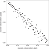 |
Figure 2 Scatter plot of the pseudo-observations. |
The 3 commands, indepTest(), exchTest() and radSymTest(), are coming from copula R-package,1 each of them allows verifying the compatibility of the models with the data. In order to guarantee some conditions, we test H 0: U and V are independent by means of the indepTest(), and H 0 is rejected with p-value < 0.001. A rather desirable property of dependence is the exchangeability, a condition required by many families of copulas including the Archimedean and the elliptical ones. So, we test H 0: U and V are exchangeable (C(u, v) = C(v, u)), using the exchTest(), see [6], and H 0 is not rejected, with p-value = 0.2562. The radial symmetry (important characteristic of Frank family) was tested by the command radSymTest() (see [7]), with H 0: there is radial symmetry, the test returns a p-value = 0.1593, indicating the possibility of this property being valid for the data.
In order to define the appropriate copula we use the copula R-package, and the function fitCopula(), with arguments (a) copula and (b) method with (a) “FrankCopula(dim = 2)”, “GaussianCopula(dim = 2)”, “tCopula(dim = 2)” and (b) method = “mpl” (maximum pseudo likelihood) which is the maximum log-likelihood (MLL) method evaluated on the pseudo observations. That is, given a copula C its density c is computed and the log-likelihood is given by  which is maximized in the underlying parameters to obtain
  , related to the model C and the set
  . Note that 2 of these models have 1 parameter while the t-Student copula model has 2 parameters, so a penalty is applied to the models in order to promote a fairer selection. We consider the Bayesian Information Criterion (BIC) for this purpose, see [2].
 (4)where N is the total number of parameters of C, and n = 96 in the dataset. According to the BIC, the higher the value taken by the equation (4), the better the model.
In the following subsection we show the results of the model selection procedure and the classical and Bayesian estimation of its parameters.
Results
We note that the two best models (copulas) are Frank and Gaussian, see Table 1. In this selection we have considered a classical estimation perspective, but we also show its Bayesian versions that give our results greater flexibility.
Parameter estimate by Maximum Pseudo Likelihood Method and BIC value for the copula between the pseudo-observations ranks (X 1) and ranks (X 2).
In Table 2 we show the results of the Bayesian analysis. We apply Hamiltonian Monte Carlo (HMC) simulations through the rstan R-package in two settings (i) a Non-informative (NI) setting and (ii) an Informative (I) setting, using in both situations the Frank and Gaussian copulas as indicated by the BIC, see Table 1. Regarding the Frank model, for (i) we use an improper prior distribution on θ (proportional to a constant), for (ii) we use a Gaussian distribution on θ, with mode equal to −25.832 and standard deviation equal to 5. Regarding the Gaussian model, for (i) we use a non-informative prior distribution on ρ (proportional to a constant), for (ii) we use a Transformed Beta distribution −1 + 2B, where B ~ Beta(1.8; 58), on ρ with mode equal to −0.974. For settings (ii) the mode of the prior distribution was built through the funcion iTau() of copula R package (moment method). For instance, by means of the empirical estimation of Kendall’s tau coefficient we can obtain an estimation of the parameter, used in those settings as mode of the prior distribution.
Summaries of the Bayesian estimation.
As expected, considering the NI settings, the Bayesian estimators under quadratic/multi linear loss function (Tab. 2 in bold) offer very close values of classical estimates, see Table 1-column 2. This evidence strengthens our confidence in the adjustments found. The I settings show how the posterior distribution would be affected with a prior distribution build with excessive influence of the observations.
Below on Figures 3b and 4b one can see the influence of these prior distributions on the posterior distributions of θ and ρ, the grey lines representing the non-informative prior and the black lines the informative prior distribution based on the Gaussian distribution (Fig. 3) and on the Transformed Beta distribution (Fig. 4). The traces plotted in Figures 3a and 4a indicate that the chains converged, as no sign of nonstationarity, no patterns as several consecutive simulations in either direction nor several equal simulations on both graphs is seen. This white-noise similar pattern is the expected one in case of convergence.
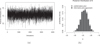 |
Figure 3 Convergence diagnostics of the HMC simulations – Frank Copula. (a) Trace plot of simulations. (b) Effect of the prior distribution. |
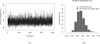 |
Figure 4 Convergence diagnostics of the HMC simulations – Gaussian Copula. (a) Trace plot of simulations. (b) Effect of the prior distribution. |
Expected value for age at death
Once the best copula model for the data is chosen, one can estimate quantities of interest that quantify the inequality between race and life expectancy upon analysing, for instance, first based on the pseudo-observations, ![Mathematical equation: $ \mathbb{E}(V|U\in (a,b])$](/articles/fopen/full_html/2020/01/fopen200008/fopen200008-eq25.gif) , the mean life expectancy given the share of black and brown people in the whole neighbourhood population belongs to a specific interval (a, b] as,
, the mean life expectancy given the share of black and brown people in the whole neighbourhood population belongs to a specific interval (a, b] as,
![Mathematical equation: $$ \mathbb{E}(V|U\in \left(a,b\right])={\int }_0^1 v{c}_{V|U\in (a,b]}(v)\mathrm{d}v, $$](/articles/fopen/full_html/2020/01/fopen200008/fopen200008-eq26.gif) (5)where c
V|U∈(a,b] (⋅) denotes the conditional density of the random variable V|U ∈ (a, b], which by definition is,
(5)where c
V|U∈(a,b] (⋅) denotes the conditional density of the random variable V|U ∈ (a, b], which by definition is,
![Mathematical equation: $$ \mathrm{Prob}\enspace (V\le v|U\in (a,b])={\int }_0^v {c}_{V|U\in (a,b]}(w)\mathrm{d}w. $$](/articles/fopen/full_html/2020/01/fopen200008/fopen200008-eq27.gif) (6)
(6)
Note that both equations (5) and (6) depend on the underlying copula parameter (θ for Frank and ρ for Gaussian). We avoid incorporating the parameter in order to simplify the notation.
The conditional expectation ![Mathematical equation: $ \mathbb{E}(V|U\in (a,b])$](/articles/fopen/full_html/2020/01/fopen200008/fopen200008-eq28.gif) allows us to restrict the problem to cases by percentage bands, that is, if U ∈ (a, b], we are considering the pseudo-observations of pct proportions between a and b, under this assumption a natural question is, what is the life expectancy? To answer this, we must first compute and estimate equation (5), what we do in the following way,
allows us to restrict the problem to cases by percentage bands, that is, if U ∈ (a, b], we are considering the pseudo-observations of pct proportions between a and b, under this assumption a natural question is, what is the life expectancy? To answer this, we must first compute and estimate equation (5), what we do in the following way,
![Mathematical equation: $$ \mathrm{Prob}\enspace (V\le v|U\in (a,b])=\frac{C(b,v)-C(a,v)}{b-a}, $$](/articles/fopen/full_html/2020/01/fopen200008/fopen200008-eq29.gif) (7)and from equations (6) and (7), we have,
(7)and from equations (6) and (7), we have,
![Mathematical equation: $$ {c}_{V|U\in (a,b]}(v)=\frac{\mathrm{d}}{\mathrm{d}v}\left\{\frac{C(b,v)-C(a,v)}{b-a}\right\}. $$](/articles/fopen/full_html/2020/01/fopen200008/fopen200008-eq30.gif) (8)
(8)
Due to integration by parts, it is verified that,
 (9)
(9)
We can finally compute ![Mathematical equation: $ \mathbb{E}(V|U\in (a,b])$](/articles/fopen/full_html/2020/01/fopen200008/fopen200008-eq32.gif) ,
,
![Mathematical equation: $$ \begin{array}{cc}\mathbb{E}(V|U\in (a,b])& \stackrel{(5),(8)}{=}\frac{1}{b-a}\left({\int }_0^1 v\frac{\mathrm{d}}{\mathrm{d}v}\left\{C\left(b,v\right)\right\}\mathrm{d}v-{\int }_0^1 v\frac{\mathrm{d}}{\mathrm{d}v}\left\{C\left(a,v\right)\right\}\mathrm{d}v\right)\\ & \stackrel{(9)}{=}\frac{1}{b-a}\left(b-{\int }_0^1 C(b,v)\mathrm{d}v-a+{\int }_0^1 C(a,v)\mathrm{d}v\right)\\ & =1-\frac{1}{b-a}\left({\int }_0^1 C(b,v)\mathrm{d}v-{\int }_0^1 C(a,v)\mathrm{d}v\right).\end{array} $$](/articles/fopen/full_html/2020/01/fopen200008/fopen200008-eq33.gif) (10)
(10)
As mentioned above, C depends on the parameter, then strictly speaking the equation (10) is,
![Mathematical equation: $$ \mathbb{E}(V|U\in \left(a,b\right])=1-\frac{1}{b-a}\left({\int }_0^1 C(b,v|\theta )\mathrm{d}v-{\int }_0^1 C\left(a,v,\theta \right)\mathrm{d}v\right), $$](/articles/fopen/full_html/2020/01/fopen200008/fopen200008-eq34.gif) (11)for the Frank copula, and,
(11)for the Frank copula, and,
![Mathematical equation: $$ \mathbb{E}(V|U\in \left(a,b\right])=1-\frac{1}{b-a}\left({\int }_0^1 C(b,v|\rho )\mathrm{d}v-{\int }_0^1 C(a,v|\rho )\mathrm{d}v\right), $$](/articles/fopen/full_html/2020/01/fopen200008/fopen200008-eq35.gif) (12)for the Gaussian copula.
(12)for the Gaussian copula.
As an illustration we show in Figure 5, ![Mathematical equation: $ \mathbb{E}(V|U\in (a,b]))$](/articles/fopen/full_html/2020/01/fopen200008/fopen200008-eq36.gif) (Eqs. (11) and (12)) coming from m = 4000 simulations of θ (or ρ) using the posterior distributions built from Non Informative (NI) and Informative (I) settings, as described previously. Figure 5 shows the results for both models, Frank and Gaussian copulas. Based on the results it is possible to see the small effect of the prior distribution in the reduction of uncertainty regarding
(Eqs. (11) and (12)) coming from m = 4000 simulations of θ (or ρ) using the posterior distributions built from Non Informative (NI) and Informative (I) settings, as described previously. Figure 5 shows the results for both models, Frank and Gaussian copulas. Based on the results it is possible to see the small effect of the prior distribution in the reduction of uncertainty regarding ![Mathematical equation: $ \mathbb{E}(V|U\in (a,b])$](/articles/fopen/full_html/2020/01/fopen200008/fopen200008-eq37.gif) .
.
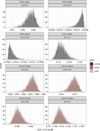 |
Figure 5 Conditional expectation, from equations (11) and (12) with θ (and ρ) simulated from the posterior distributions (non-informative and informative settings). |
For the Frank copula we estimate equation (11) by means of the Bayesian estimator by quadratic loss function of θ, say  ,
,
![Mathematical equation: $$ \widehat{\mathbb{E}}(V|U\in (a,b])=1-\frac{1}{b-a}\left({\int }_0^1 C(b,v|{\widehat{\theta }}_B)\mathrm{d}v-{\int }_0^1 C(a,v|{\widehat{\theta }}_B)\mathrm{d}v\right). $$](/articles/fopen/full_html/2020/01/fopen200008/fopen200008-eq39.gif) (13)
(13)
In the same way for the Gaussian copula we estimate (12) by means of the Bayesian estimator by quadratic loss function of ρ, say  ,
,
![Mathematical equation: $$ \widehat{\mathbb{E}}(V|U\in \left(a,b\right])=1-\frac{1}{b-a}\left({\int }_0^1 C(b,v|{\widehat{\rho }}_B)\mathrm{d}v-{\int }_0^1 C(a,v|{\widehat{\rho }}_B)\mathrm{d}v\right). $$](/articles/fopen/full_html/2020/01/fopen200008/fopen200008-eq41.gif) (14)
(14)
The estimator given by equation (13) and (14) is evaluated upon simulated (of size m = 4000)  (and
(and  ) from the posterior distribution for each combination of copula model2 and prior distribution.3 The results are in Table 3.
 , i = 1, 2 are computed using Frank copula,
  , i = 3, 4 are computed using Gaussian copula, i = 1, 3 from Informative settings, i = 2, 4 from Non Informative settings. In bold the lowest values per line.


Given each interval (a, b] the estimates are very close regardless of the copula (and prior distribution) used to compute the conditional expectation (see each line of Tab. 3). This shows that the conditional expectation is capable of neutralizing the effect visualized in Figure 5. As the data indicates, without giving a precise magnitude that now we have, as the percentage of pct increases, life expectancy decreases. The table also gives us in what percentages the decreasing occurs. The conditional means show a mean decrease at a proportional rate from one stratum to another, since for example, the difference between ![Mathematical equation: $ {\widehat{\mathbb{E}}}_1(V|U\in (0,\mathrm{\enspace }0.25])$](/articles/fopen/full_html/2020/01/fopen200008/fopen200008-eq44.gif) and
and ![Mathematical equation: $ {\widehat{\mathbb{E}}}_1(V|U\in (0.25,\mathrm{\enspace }0.5])$](/articles/fopen/full_html/2020/01/fopen200008/fopen200008-eq45.gif) is 0.24, between
is 0.24, between ![Mathematical equation: $ {\widehat{\mathbb{E}}}_1(V|U\in (0.25,\mathrm{\enspace }0.5])$](/articles/fopen/full_html/2020/01/fopen200008/fopen200008-eq46.gif) and
and ![Mathematical equation: $ {\widehat{\mathbb{E}}}_1(V|U\in (0.5,\mathrm{\enspace }0.75])$](/articles/fopen/full_html/2020/01/fopen200008/fopen200008-eq47.gif) is 0.25 and between
is 0.25 and between ![Mathematical equation: $ {\widehat{\mathbb{E}}}_1(V|U\in (0.5,\mathrm{\enspace }0.75])$](/articles/fopen/full_html/2020/01/fopen200008/fopen200008-eq48.gif) and
and ![Mathematical equation: $ {\widehat{\mathbb{E}}}_1(V|U\in (0.75,\mathrm{\enspace }1])$](/articles/fopen/full_html/2020/01/fopen200008/fopen200008-eq49.gif) is 0.24.
is 0.24.
The evidence indicated by Table 3 could lead us to the conclusion that the curves’ performances (from Eqs. (11) to (12)) are identical, for each of the bands (a, b], except for a displacement at a rate of approximately 0.25, but this is not true. For instance, for the Frank copula (best model according to Tab. 1) and under the non informative setting we can see that the curves show in the extreme intervals (0,0.25] and (0.75,1] a greater dispersion in comparison with the curves for the central intervals, as can be seen based on Table 4, which presents the interquartile ranges of the conditional expectations. Furthermore, the 4 curves are quite different in terms of symmetry/asymmetry. For further details and information, see [8]. This study leads to the need to deepen the investigation, in the framework of each of these situations (a, b], since other factors could explain the performance of these curves, such as purchasing power, access to health care, educational level, criminality level, access to clean water and correct disposal of sewage, etc.
Conclusions
The models of copulas are useful to describe the dependence between variables (see [1]), and as has been done in this paper, they are tools for analyzing implications and impacts on social realities. In this study we have combined two powerful tools, the copula models and the Bayesian estimation. With such tools we have been able to inspect the relationship between (i) pct proportion of the black/brown population in relation to the total population of the neighborhood and (ii) age average age at which people died in the neighborhood. Assuming different perspectives, through copula models pointed out by the BIC – see [2] and, informative/non-informative settings we can fully describe the relationship by exercising different theoretical assumptions (see Tabs. 1 and 2). This diversity of scenarios finds common points for the estimation of life expectancy conditioned at pct percentile intervals (see Tab. 3). And it also offers ways to compare the results. The non-informative scenario and Frank’s copula [5] are then established as the starting point for future inspections, in relation to which future results could be compared, or results obtained after certain social events that may alter performance between pct and age.
We see that for the specific database discussed here (as of 2018) the state of São Paulo shows life expectancies that fall with increasing pct percentages. On average, the fall rate is constant and decreases as the percentage interval of pct (a, b] increases, a, b ∈ [0, 1]. In other words, since we have set 4 referential intervals for the proportions of pct, from (0, 0.25] to (0.25, 0.5] we have a rate of fall in life expectancy of around 0.25 (scale from 0 to 1) that is repeated em the fall in life expectancy for proportions of pct from (0.25, 0.5] to (0.5, 0.75] and also for proportions of pct from (0.5, 0.75] to (0.75, 1]. Furthermote, when observing the life expectancy in each of these intervals, Figure 5, we verify that depending on the interval the curve shows a markedly different performance, which leads us to other questions such as what are the factors that determine each specific behaviour? Those questions are outside of our focus but certainly are very relevant for future studies.
Acknowledgments
R. Rodrigues de Moraes gratefully acknowledge the partial financial support provided by CAPES with a fellowship from the Master Program in Statistics – University of Campinas. We thank the editor who led the review process, for their many helpful comments and suggestions on an earlier draft of this paper.
Frank copula and Gaussian copula.
Gaussian prior for Frank copula, Transformed Beta prior for the Gaussian copula.
References
- Nelsen RB (2007), An introduction to copulas, Springer Science & Business Media. [Google Scholar]
- Schwarz G (1978), Estimating the dimension of a model. Ann Stat 6, 2, 461–464. [Google Scholar]
- Sklar M (1959), Fonctions de repartition an dimensions et leurs marges. Publ Inst Statist Univ Paris 8, 229–231. [Google Scholar]
- Mikusinski P, Sherwood H, Taylor MD (1991), The Fréchet bounds revisited. Real Anal Exch 17, 2, 759–764. [CrossRef] [Google Scholar]
- Frank MJ (1979), On the simultaneous associativity of F(x, y) and x + y − F(x, y). Aequ Math 19, 1, 194–226. [Google Scholar]
- Genest C, Nešlehová J (2012), Tests of symmetry for bivariate copulas. Ann Inst Stat Math 64, 4, 811–834. [Google Scholar]
- Genest C, Nešlehová J (2014), On tests of radial symmetry for bivariate copulas. Stat Papers 55, 4, 1107–1119. [CrossRef] [Google Scholar]
- Rodrigues de Moraes R (2020), Eventos Caudais na Prática. Modelagem Bayesiana via Cópulas (Unpublished Master’s Thesis). [Google Scholar]
Cite this article as: González-López VA & Rodrigues de Moraes R 2020. A copula-based quantifying of the relationship between race inequality among neighbourhoods in São Paulo and age at death. 4open, 3, 11
All Tables
Parameter estimate by Maximum Pseudo Likelihood Method and BIC value for the copula between the pseudo-observations ranks (X 1) and ranks (X 2).
, i = 1, 2 are computed using Frank copula, , i = 3, 4 are computed using Gaussian copula, i = 1, 3 from Informative settings, i = 2, 4 from Non Informative settings. In bold the lowest values per line.
All Figures
|
Figure 1 Dependence structure in the race inequality between neighbourhoods in São Paulo. (a) Scatter plot of observations. (b) The 25 cases with the highest proportion of white population. (c) The 25 cases with the highest proportion of black/brown population. |
| In the text | |
|
Figure 2 Scatter plot of the pseudo-observations. |
| In the text | |
|
Figure 3 Convergence diagnostics of the HMC simulations – Frank Copula. (a) Trace plot of simulations. (b) Effect of the prior distribution. |
| In the text | |
|
Figure 4 Convergence diagnostics of the HMC simulations – Gaussian Copula. (a) Trace plot of simulations. (b) Effect of the prior distribution. |
| In the text | |
|
Figure 5 Conditional expectation, from equations (11) and (12) with θ (and ρ) simulated from the posterior distributions (non-informative and informative settings). |
| In the text | |