| Issue |
4open
Volume 2, 2019
Advances in Researches of Quaternion Algebras
|
|
|---|---|---|
| Article Number | 16 | |
| Number of page(s) | 7 | |
| Section | Mathematics - Applied Mathematics | |
| DOI | https://doi.org/10.1051/fopen/2019014 | |
| Published online | 05 June 2019 | |
Research Article
Eigenvalues of matrices related to the octonions
1
Departamento de Matemática and CMA-UBI, Universidade da Beira Interior, 6201-001 Covilhã, Portugal
2
Departamento de Matemática, Universidade de Coimbra, 3004-531 Coimbra, Portugal
* Corresponding author: This email address is being protected from spambots. You need JavaScript enabled to view it.
Received:
29
December
2018
Accepted:
20
April
2019
Abstract
A pseudo real matrix representation of an octonion, which is based on two real matrix representations of a quaternion, is considered. We study how some operations defined on the octonions change the set of eigenvalues of the matrix obtained if these operations are performed after or before the matrix representation. The established results could be of particular interest to researchers working on estimation algorithms involving such operations.
Mathematics Subject Classification: 11R52 / 15A18
Key words: Octonions / Quaternions / Real matrix representations / Eigenvalues
© R. Serôdio et al., Published by EDP Sciences, 2019
 This is an Open Access article distributed under the terms of the Creative Commons Attribution License (http://creativecommons.org/licenses/by/4.0/), which permits unrestricted use, distribution, and reproduction in any medium, provided the original work is properly cited.
1 Introduction
Due to nonassociativity, the real octonion division algebra is not algebraically isomorphic to a real matrix algebra. Despite this fact, pseudo real matrix representations of an octonion may be introduced, as in [1], through real matrix representations of a quaternion.
In this work, the left matrix representation of an octonion over  , as called by Tian in [1], is considered. For the sake of completeness, some definitions and results, in particular on this pseudo representation, are recalled in Section 2.
Using the mentioned representation, results concerning eigenvalues of matrices related to the octonions are established in Section 3. Previous research on this subject, although not explicitly applying real matrix representations of a quaternion, can be seen in [2].
2 Real octonion division algebra
Consider the real octonion division algebra  , that is, the usual real vector space
  , with canonical basis
  , equipped with the multiplication given by the relations
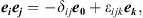 where δ
ij
is the Kronecker delta, ε
ijk
is a Levi-Civita symbol, i.e., a completely antisymmetric tensor with a positive value +1 when ijk = 123, 145, 167, 246, 275, 374, 365 and
e
0
is the identity. This element will be omitted whenever it is clear from the context.
where δ
ij
is the Kronecker delta, ε
ijk
is a Levi-Civita symbol, i.e., a completely antisymmetric tensor with a positive value +1 when ijk = 123, 145, 167, 246, 275, 374, 365 and
e
0
is the identity. This element will be omitted whenever it is clear from the context.
Every element
o
∈  can be written as
  where Re(
o
) = o
0 and
where Re(
o
) = o
0 and  are called the real part and the imaginary (or vector) part, respectively. The conjugate of
o
is defined as
are called the real part and the imaginary (or vector) part, respectively. The conjugate of
o
is defined as  . The norm of
o
is defined by
. The norm of
o
is defined by  . The inverse of a non-zero octonion
o
is
. The inverse of a non-zero octonion
o
is  .
.
The multiplication of  can be written in terms of the Euclidean inner product and the vector cross product in
  , hereinafter denoted by • and ×, respectively. Concretely, as in [3], we have
Following [4], we recall that  are perpendicular if
  . In particular, if
  , then
  are perpendicular if
  . Moreover,
  are parallel if
  . In particular, if
  , then
  are parallel if
  .
.
The elements of the basis of  can also be written as
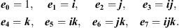
The real octonion division algebra  , of dimension 8, can be constructed from the real quaternion division algebra
  , of dimension 4, by the Cayley-Dickson doubling process where
  contains
  as a subalgebra. As a consequence, it is well known that any
  can be written as
  (1) where
  are of the form
  , with
  .
.
The real quaternion division algebra  is algebraically isomorphic to the real matrix algebra of the matrices in (2), where ϕ(q) is a real matrix representation of a quaternion q.
Definition 1
[1] Let  . Then
![Mathematical equation: $$ \phi (q)=\left[\begin{array}{llll}{q}_0& -{q}_1& -{q}_2& -{q}_3\\ {q}_1& {q}_0& -{q}_3& {q}_2\\ {q}_2& {q}_3& {q}_0& -{q}_1\\ {q}_3& -{q}_2& {q}_1& {q}_0\end{array}\right]. $$](/articles/fopen/full_html/2019/01/fopen180050/fopen180050-eq38.gif) (2)
(2)
Some important properties of the matrices in Definition 1 are recalled in Lemma 1.
Lemma 1
[1] Let  and
and  . Then
-
 .
. -
 .
. -
 .
. -
 , if
, if  .
. -
![Mathematical equation: $ \mathrm{det}\left[\phi (a)\right]=|a{|}^4$](/articles/fopen/full_html/2019/01/fopen180050/fopen180050-eq46.gif) .
.
The real quaternion division algebra  is algebraically anti-isomorphic to the real matrix algebra of the matrices in (3), where τ(q) is another real matrix representation of a quaternion q.
Definition 2
[1] Let  . Then
![Mathematical equation: $$ \tau (q)={K}_4{\phi }^T(q){K}_4=\left[\begin{array}{llll}{q}_0& -{q}_1& -{q}_2& -{q}_3\\ {q}_1& {q}_0& {q}_3& -{q}_2\\ {q}_2& -{q}_3& {q}_0& {q}_1\\ {q}_3& {q}_2& -{q}_1& {q}_0\end{array}\right], $$](/articles/fopen/full_html/2019/01/fopen180050/fopen180050-eq49.gif) (3) where K4 = diag(1, −1, −1, −1).
(3) where K4 = diag(1, −1, −1, −1).
Some relevant properties of the matrices in Definition 2 are recalled in Lemma 2.
Lemma 2
[1] Let  and
and  . Then
-
 .
. -
τ(a + b) = τ(a) + τ(b), τ(ab) = τ(b)τ(a), τ(λa) = λτ(a), τ(1) = I 4.
-
 .
. -
 , if
, if  .
. -
![Mathematical equation: $ \mathrm{det}\left[\tau (a)\right]=|a{|}^4$](/articles/fopen/full_html/2019/01/fopen180050/fopen180050-eq56.gif) .
.
Due to the non-associativity, the octonion algebra cannot be isomorphic to the real matrix algebra with the usual multiplication. With the purpose of introducing a convenient matrix multiplication, we show another way of representing the octonions by a column matrix.
Definition 3
Let 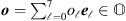 . The column
, vectorial or ket representation of
o
is
. The column
, vectorial or ket representation of
o
is ![Mathematical equation: $ |{o}\right\rangle=[{o}_0\enspace {o}_1\enspace \cdots \enspace {o}_7{]}^T$](/articles/fopen/full_html/2019/01/fopen180050/fopen180050-eq58.gif) .
.
Based on the previous real matrix representations of a quaternion, Tian introduced the following pseudo real matrix representation of an octonion.
Definition 4
[1] Let  , where
  . Then the 8 × 8 real matrix
![Mathematical equation: $$ \omega ({a})=\left[\begin{array}{ll}\phi (a\mathrm{\prime})& -\tau ({a}^{\prime\prime }){K}_4\\ \phi ({a}^{\prime\prime }){K}_4& \tau (a\mathrm{\prime})\end{array}\right], $$](/articles/fopen/full_html/2019/01/fopen180050/fopen180050-eq61.gif) (4) is called the left matrix representation of
a
over
(4) is called the left matrix representation of
a
over  , where K
4 = diag(1, −1, −1, −1).
, where K
4 = diag(1, −1, −1, −1).
The meaning of the term left matrix representation comes from the following result.
Theorem 1
[1] Let  . Then
  .
.
Tian [1] introduced also the right matrix representation of an octonion
a
over  , which he denoted by
  . In this case, Tian proved that
  .
.
Even though there are  such that
  , there are still some properties which hold. These are recalled in Theorem 2.
Theorem 2
[1] Let  ,
,  . Then
-
 .
. -
ω( a + b ) = ω( a ) + ω( b ), ω(λ a ) = λω( a ), ω(1) = I 8.
-
 .
.
3 Main results
In this section, the left matrix representation of an octonion over  is considered. First of all, given an octonion, the eigenvalues of its left matrix representation are computed.
Proposition 1
Let  . Then the eigenvalues of the real matrix ω(
a
) are
. Then the eigenvalues of the real matrix ω(
a
) are
 each with algebraic multiplicity 4.
Proof. Given an octonion a, it can always be uniquely represented as  such that
  , and where
  . The characteristic polynomial of ω(
a
) is
. The characteristic polynomial of ω(
a
) is  where K
8 is the orthogonal matrix diag(1, −1, −1, −1, 1, 1, 1, 1) = diag(K
4, I
4). Hence,
where K
8 is the orthogonal matrix diag(1, −1, −1, −1, 1, 1, 1, 1) = diag(K
4, I
4). Hence, ![Mathematical equation: $$ \mathrm{det}(\lambda {I}_8-\omega ({a}))=\mathrm{det}\left(\left[\begin{array}{ll}{K}_4& 0\\ 0& {I}_4\end{array}\right]\left[\begin{array}{ll}\phi (\lambda -{a}_0-a\mathrm{\prime})& \tau ({a}^{\prime\prime }){K}_4\\ -\phi (a\mathrm{\prime}\mathrm{\prime}){K}_4& \tau (\lambda -{a}_0-a\mathrm{\prime})\end{array}\right]\left[\begin{array}{ll}{K}_4& 0\\ 0& {I}_4\end{array}\right]\right) $$](/articles/fopen/full_html/2019/01/fopen180050/fopen180050-eq81.gif)
![Mathematical equation: $$ =\mathrm{det}\left[\begin{array}{ll}\tau (\lambda -{a}_0+a\mathrm{\prime})& \mathrm{\phi }(\overline{{a}^{\prime\prime }})\\ -\mathrm{\phi }({a}^{\prime\prime })& \tau (\lambda -{a}_0-a\mathrm{\prime})\end{array}\right] $$](/articles/fopen/full_html/2019/01/fopen180050/fopen180050-eq82.gif)


 and the result follows.
The set of eigenvalues of ω( ab ) is equal to the set of eigenvalues of ω( a )ω( b ) since the characteristic polynomials are equal as can easily be seen. However, if we add an extra octonion c the set of eigenvalues of ω( ab + c ) and ω( a )ω( b ) + ω( c ) may differ.
We now study the eigenvalues of the matrix ω( a )ω( b ) + ω( c ), given three octonions a , b , and c .
Remark 1
Let 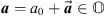 and
and  . Notice that
  can be decomposed into two parts: a part parallel to
  , denoted by
  ; and a part perpendicular to
  , denoted by
  . The parallel part is the projection of
  onto
onto  , which is defined as
 The perpendicular part is given by
  .
.
Besides the projection of  onto
onto  we will also consider the projection of
  over
over  , i.e., the linear space generated by all linear combinations of
  and
and  .
.
Remark 2
As  and
and  , then
 where
where  and
and  . Hence, it suffices to consider only the product
  since the remaining terms can be added to
c
.
since the remaining terms can be added to
c
.
The pure octonion  can be decomposed in two parts, one in
  and the other perpendicular to it. In this case, we can write
  , where
  and
and  . The parallel part is the projection of
  onto
onto  and is given by
 and the perpendicular part is naturally
  .
.
Proposition 2
Let  such that
  , and the imaginary part of
a
and
b
are perpendicular. Then the eigenvalues of the real matrix ω(
a
)ω(
b
) + ω(
c
) are
, and the imaginary part of
a
and
b
are perpendicular. Then the eigenvalues of the real matrix ω(
a
)ω(
b
) + ω(
c
) are
 (5)
where
c
∥ is the projection of
c
onto Span(
a
,
b
) and
(5)
where
c
∥ is the projection of
c
onto Span(
a
,
b
) and  , each with algebraic multiplicity 2.
Proof. Without loss of generality, we consider
a
= a
i
and
b = b
j
. Hence, ![Mathematical equation: $$ \begin{array}{cc}\omega \left({a}\right)\omega \left({b}\right)& =\left[\begin{array}{ll}\phi \left(a{i}\right)& 0\\ 0& \tau \left(a{i}\right)\end{array}\right]\left[\begin{array}{ll}\phi \left(b{j}\right)& 0\\ 0& \tau \left(b{j}\right)\end{array}\right]\\ & =\left[\begin{array}{ll}\phi (a{i})\phi (b\mathbf{j})& 0\\ 0& \tau (a\mathbf{i})\tau (b\mathbf{j})\end{array}\right]\end{array}. $$](/articles/fopen/full_html/2019/01/fopen180050/fopen180050-eq124.gif)
By Lemmas 1 and 2, we have ![Mathematical equation: $$ \omega ({a})\omega ({b})=\left[\begin{array}{ll}\phi ({ab}{ij})& 0\\ 0& \tau (-{ab}{ij})\end{array}\right]. $$](/articles/fopen/full_html/2019/01/fopen180050/fopen180050-eq125.gif) (6) Let
(6) Let  , where
  . Then
 ![Mathematical equation: $$ \omega ({c})=\left[\begin{array}{ll}\phi ({c}_0+{c}_1{i}+{c}_2{j}+{c}_3{ij})& -\tau ({c}^{\prime\prime }){K}_4\\ \phi ({c}^{\prime\prime }){K}_4& \tau ({c}_0+{c}_1{i}+{c}_2{j}+{c}_3{ij})\end{array}\right]. $$](/articles/fopen/full_html/2019/01/fopen180050/fopen180050-eq128.gif) (7)
(7)
Taking into account (6) and (7), we obtain ![Mathematical equation: $$ \omega \left({a}\right)\omega \left({b}\right)+\omega \left({c}\right)=\left[\begin{array}{ll}\phi \left({c}_0+{c}_1{i}+{c}_2{j}+\left({c}_3+{ab}\right){ij}\right)& -\tau \left({c}^{\prime\prime }\right){K}_4\\ \phi \left({c}^{\prime\prime }\right){K}_4& \tau \left({c}_0+{c}_1{i}+{c}_2{j}+\left({c}_3-{ab}\right){ij}\right)\end{array}\right]. $$](/articles/fopen/full_html/2019/01/fopen180050/fopen180050-eq129.gif)
The characteristic polynomial of ω(
a
)ω(
b
) + ω(
c
) is  where K8 is the orthogonal matrix diag(1, −1, −1, −1, 1, 1, 1, 1) = diag(K
4, I
4). Hence,
where K8 is the orthogonal matrix diag(1, −1, −1, −1, 1, 1, 1, 1) = diag(K
4, I
4). Hence, ![Mathematical equation: $$ p(\lambda )=\mathrm{det}\left[\begin{array}{ll}\tau ({c}_0-\lambda -{c}_1{i}-{c}_2{j}-({c}_3+{ab}){ij})& -\phi (\overline{{c}^{\prime\prime }})\\ \phi ({c}^{\prime\prime })& \tau ({c}_0-\lambda +{c}_1{i}+{c}_2{j}+({c}_3-{ab}){ij})\end{array}\right], $$](/articles/fopen/full_html/2019/01/fopen180050/fopen180050-eq131.gif) which results in
which results in  and, since
  , gives
  where
where  and
and  . By Lemma 2, we have
 ![Mathematical equation: $$ \begin{array}{cc}p(\lambda )& ={\left[(({c}_0-\lambda {)}^2+|{\mathbf{c}}_{\parallel }{|}^2+|{\mathbf{c}}_{\perp }{|}^2-({ab}{)}^2{)}^2+4({ab}{)}^2(|{\mathbf{c}}_{\parallel }{|}^2+({c}_0-\lambda {)}^2)\right]}^2\\ & \begin{array}{c}=\left[(({c}_0-\lambda {)}^2+|{\mathbf{c}}_{\parallel }{|}^2{)}^2+2(({c}_0-\lambda {)}^2+|{\mathbf{c}}_{\parallel }{|}^2)(|{\mathbf{c}}_{\perp }{|}^2-({ab}{)}^2)+(|{\mathbf{c}}_{\perp }{|}^2-({ab}{)}^2{)}^2\right.+{\left.4({ab}{)}^2(|{\mathbf{c}}_{\parallel }{|}^2+({c}_0-\lambda {)}^2)\right]}^2\\ =\left[(({c}_0-\lambda {)}^2+|{\mathbf{c}}_{\parallel }{|}^2{)}^2+2(({c}_0+\lambda {)}^2+|{\mathbf{c}}_{\parallel }{|}^2)(|{\mathbf{c}}_{\perp }{|}^2-({ab}{)}^2)+(|{\mathbf{c}}_{\perp }{|}^2({ab}{)}^2{)}^2-\right.{\left.4({ab}{)}^2|{\mathbf{c}}_{\perp }{|}^2\right]}^2\end{array}\\ & \begin{array}{c}={\left[(({c}_0-\lambda {)}^2+|{\mathbf{c}}_{\parallel }{|}^2+|{\mathbf{c}}_{\perp }{|}^2+({ab}{)}^2{)}^2-4({ab}{)}^2|{\mathbf{c}}_{\perp }{|}^2\right]}^2\\ ={\left[(({c}_0-\lambda {)}^2+|\overrightarrow{{c}}{|}^2+({ab}{)}^2{)}^2-4({ab}{)}^2|{\mathbf{c}}_{\perp }{|}^2\right]}^2,\end{array}\end{array} $$](/articles/fopen/full_html/2019/01/fopen180050/fopen180050-eq137.gif) and the result follows.
and the result follows.
The following corollary may be useful to improve the localization of eigenvalues of octonionic matrices and zeros of octonionic polynomials whenever such products occur.
Corollary 2.1
Let  . Then
 (8) where ρ(•) stands for the spectral radius.
Proof. By Proposition 2, we obtain 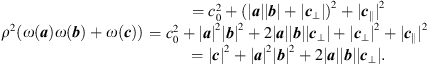
Furthermore, the eigenvalues of ω(
ab +
c
) are all equal in modulus and satisfy 
Without loss of generality, we can consider
a
= a
i
and
b
= b
j
. If  . Hence, we arrive at
  and the result follows.
Example 3.1
Let 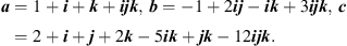
To apply (5)
, we have to take into account Remarks 1 and 2, and rewrite
a
,
b
and
c
as
 where
where  ,
,  and
and  are the imaginary parts of
a
,
b
and
c
, respectively.
are the imaginary parts of
a
,
b
and
c
, respectively.
Computing  , the projection of
  onto
onto  , we obtain
  . Thus, the orthogonal part
  is equal to
  .
.
The projections of  onto
onto  and
and  are, respectively
  and
and  . Hence, the projection of
  on the space of
  and
and  is
is  . This implies that for the orthogonal part we have
  .
.
Taking all together, we have

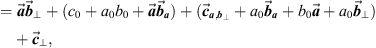 where
where  is real and
  . So
. So
 (9) where
  ,
,  , and
, and  .
.
We are now in condition to apply Proposition 2, from which we obtain the eigenvalues of
![Mathematical equation: $$ \omega ({a})\omega ({b})+\omega ({c})=\left[\begin{array}{cccccccc}-2& 1& 0& -5& -4& 6& -4& 12\\ -1& -2& 1& -2& 6& 0& -8& -4\\ 0& -1& -2& -1& 2& 8& -2& -6\\ 5& 2& 1& -2& 12& -2& 6& 2\\ 4& -6& -2& -12& -2& 1& -2& -5\\ -6& 0& -8& 2& -1& -2& -1& -4\\ 4& 8& -2& -6& 2& 1& -2& 1\\ -12& 4& 6& -2& 5& 4& -1& -2\end{array}\right]. $$](/articles/fopen/full_html/2019/01/fopen180050/fopen180050-eq173.gif)
The eigenvalues are  and
and  , while the eigenvalues of
  are
are 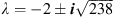 .
.
As predicted by Corollary 2.1,  , since
  and
and  .
.
Acknowledgments
The authors are very thankful to the anonymous referee for his valuable suggestions towards the improvement of this paper.
R. Serôdio and P.D. Beites were supported by Fundação para a Ciência e a Tecnologia (Portugal), project UID/MAT/00212/2013 of the Centro de Matemática e Aplicações da Universidade da Beira Interior (CMA-UBI). P.D. Beites was also supported by the research project MTM2017-83506-C2-2-P (Spain).
References
- Tian Y (2000), Matrix representations of octonions and their applications. Adv Appl Clifford Algebras 10, 61–90. [CrossRef] [Google Scholar]
- Beites PD, Nicolás AP, Vitória J (2017), On skew-symmetric matrices related to the vector cross product in R7. Electron J Linear Algebra 32, 138–150. [CrossRef] [Google Scholar]
- Leite FS (1993), The geometry of hypercomplex matrices. Linear Multilinear Algebra 34, 123–132. [CrossRef] [Google Scholar]
- Ward JP (1997), Quaternions and Cayley numbers, Kluwer, Dordrecht. [CrossRef] [Google Scholar]
Cite this article as: Serôdio R, Beites P & Vitória J 2019. Eigenvalues of matrices related to the octonions. 4open, 2, 16.