| Issue |
4open
Volume 2, 2019
Difference & Differential Equations and Applications
|
|
|---|---|---|
| Article Number | 17 | |
| Number of page(s) | 7 | |
| Section | Mathematics - Applied Mathematics | |
| DOI | https://doi.org/10.1051/fopen/2019009 | |
| Published online | 29 May 2019 | |
Research Article
To the theory of discrete boundary value problems
Chair of Differential Equations, Belgorod State National Research University, ul. Pobedy, 85, Belgorod 308015, Russia
* Corresponding author: This email address is being protected from spambots. You need JavaScript enabled to view it.
Received:
7
January
2019
Accepted:
5
April
2019
Abstract
We consider discrete analogues of pseudo-differential operators and related discrete equations and boundary value problems. Existence and uniqueness results for special elliptic discrete boundary value problem and comparison for discrete and continuous solutions are given for certain smooth data in discrete Sobolev–Slobodetskii spaces.
Mathematics Subject Classification: Primary: 35S15 / Secondary: 65T50
Key words: Digital pseudo-differential operator / Discrete boundary value problem / Periodic factorization / Discrete solution / Error estimate
© O.A. Tarasova & V.B. Vasilyev, Published by EDP Sciences, 2019
 This is an Open Access article distributed under the terms of the Creative Commons Attribution License (http://creativecommons.org/licenses/by/4.0/), which permits unrestricted use, distribution, and reproduction in any medium, provided the original work is properly cited.
1 Introduction
As a rule the classical pseudo-differential operator in Euclidean space  is defined by the formula [1, 2]:
 where the sign ∼ over a function denotes its Fourier transform,
 and the function
  is called a symbol of a pseudo-differential operator A.
Our main goal here is describing a periodic variant of this definition and studying its certain properties related to solvability of corresponding equations in canonical domains of an Euclidean space. In this paper the main result is related to a comparison of discrete and continuous solutions. We try to preserve maximal correspondence for discrete and continuous cases under digitization, it permits to find more appropriate constructions.
This problem is very large and in our opinion it should include the following aspects according to a lot of physical and technical applications of such operators and related equations:
-
finite and infinite discrete Fourier transform as a natural technique for such equations;
-
choice of appropriate discrete functional spaces;
-
studying solvability for infinite discrete equations;
-
studying solvability of approximating finite discrete equations;
-
a comparison between continuous and infinite discrete equations;
-
a comparison between infinite discrete and finite discrete equations.
This is not completed list of questions for studying which we intend to consider. Some results in this direction were obtained for simplest pseudo-differential operators (Calderon–Zygmund operators [3, 4]) and corresponding equations. Also certain results are related to approximate solutions.
There are few variants of the theory of discrete boundary value problems (see, for example [5, 6]), but these theories are related especially to partial differential operators and do not use the harmonic analysis technique. Since the classical theory of pseudo-differential operators is based on the Fourier transform we will use the discrete Fourier transform and discrete analogue of pseudo-differential operators which will include discrete analogues of partial differential and some integral convolution operators.
2 Discrete spaces and digital operators
2.1 Discrete Sobolev–Slobodetskii spaces
Given function u
d
of a discrete variable  , h > 0, we define its discrete Fourier transform by the series:
 where
where ![Mathematical equation: $ {\mathbb{T}}^m=[-\pi,\pi {]}^m,\enspace \mathrm{\hslash }={h}^{-1}$](/articles/fopen/full_html/2019/01/fopen190006/fopen190006-eq7.gif) , and partial sums are taken over cubes,
, and partial sums are taken over cubes,
We will remind here some definitions of functional spaces [7] and will consider discrete analogue of the Schwartz space  . Let us denote
 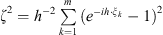 and introduce the following.
The space
 is a closure of the space
 with respect to the norm,
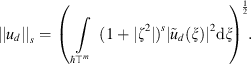 (1)
(1)
Fourier image of the space
 will be denoted by
 .
.
2.2 Digital pseudo-differential operators
One can define some discrete operators for such functions u d .
If  is a periodic function in
  with the basic cube of periods
  then we consider it as a symbol. We will introduce a digital pseudo-differential operator in the following way.
A digital pseudo-differential operator A d in a discrete domain D d is called the operator [7],
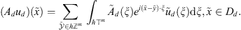
We use the class  [7] with the following condition:
 (2)and universal positive constants c
1, c
2.
(2)and universal positive constants c
1, c
2.
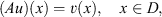
Let  be a domain. We will study the equation:
 (3)in the discrete domain
  and will seek a solution u
d
∈ H
s
(D
d
),
and will seek a solution u
d
∈ H
s
(D
d
),  [7–9].
Earlier some canonical domains [8–16] were considered but in this paper we will discuss the cases  .
.
3 Solvability and digital-periodic projectors
3.1 Periodic factorization
This case  is very different from
  , and an ellipticity condition is not sufficient for a solvability. A principal role for the solvability takes a concept of the periodic factorization which is defined for an elliptic symbol.
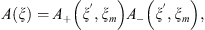
To describe a solvability picture for equation (3) we introduce the following notations. Let us denote  .
.
We will use a special periodic factorization of an elliptic symbol  :
:
 where the factors
  have some analytical properties in half-strips
  and satisfy certain estimates [7, 8].
The special index æ of periodic factorization determines the solvability for equation (3), and for special cases we will describe obtained results [7, 8]. These cases are distinct. So, if |æ − s| < 1/2 then we have the unique solution:
 (4)
(4)
 for equation (3). But if
  then there are a lot of solutions,
 where
where  is an arbitrary polynomial of order n of variables
  , satisfying the condition (2),
 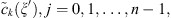 are arbitrary functions from
  .
.
3.2 Approximation schemes
We will consider the pseudo-differential equation:
 (5)and suggest for its solution some computational schemes.
We assume that the symbol  of the operator A satisfies the condition:
 (6)and it is well-known such a symbol admits factorization,
 with respect to the last variable
  with the index æ [1].
Since we know solvability conditions for pseudo-differential equations in  and
and  [1] we will select such discrete pseudo-differential operators which reserve all needed properties of their continuous analogues.
3.2.1 Equations in a whole space
Let P
h
be a restriction operator on  , i.e. for
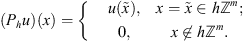
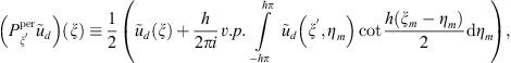
We tried this projector for simplest pseudo-differential operators, namely Calderon–Zygmund operators, these operators can be treated as pseudo-differential operators of order 0, and we obtained very acceptable results [3, 10–12]. But now we will use another restriction operator.
A construction for the restriction operator Q
h
for functions  is the following. We take the Fourier transform
  , then its restriction on
  and periodically continue it onto a whole
  . Further we apply the inverse discrete Fourier transform
  and obtain a discrete function which is denoted by
  . In our opinion the projector Q
h
is more convenient than P
h
although the projectors P
h
and Q
h
are almost the same according to the following result.
. In our opinion the projector Q
h
is more convenient than P
h
although the projectors P
h
and Q
h
are almost the same according to the following result.
For
 we have,
 where the constant C depends on u only.
Further, the symbol  will be defined in the following way. We take a restriction of
  on the cube
  and periodically extend it onto a whole
  . We consider such h-operator as an approximate operator for A. So, to find a discrete solution for equation (3) for
  we can use the following discrete equation:
 (7)
(7)
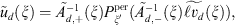
Its solution is given by the formula,
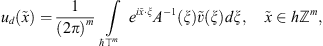 so that we do not need to find an approximate solution for an infinite system of linear algebraic equations like [3, 10]. For our case we need to apply any kind of cubature formulas for calculating the latter integral and a cubature formula for calculating the Fourier transform
  .
.
According to Lemma 1 one can compare discrete and continuous solutions for enough smooth right-hand sides and symbols.
If the symbol
 satisfies the condition and is infinitely differentiable on
 , u is a solution of the equation
(4)
, u
d
is a solution of the equation
(5)
then for
, u is a solution of the equation
(4)
, u
d
is a solution of the equation
(5)
then for
 we have the following error estimate:
 for arbitrary β > 0.
Proofs for Lemma 1 and Theorem 1 are given in [17].
3.2.2 Equations in a half-space
If we put strong enough restrictions on a right-hand side and factorization elements then one can give a comparison between discrete and continuous solutions.
If
 then the following estimate:
 holds for
  , and the constant C depends on u only.
Starting from Lemma 2 and the Theorem 1 we are able to compare discrete and continuous solutions in a half-space. Below we give this comparison under such conditions when a unique solution exists.
To formulate the following theorem we will describe how we need to choose a right-hand side for solving equation (3). We have the following solution of equation (5):
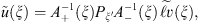 where
where 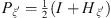 is a projector defined by the classical Hilbert transform with respect to a variable
  [1],
[1],
 is a continuation of v from
  into
into  in corresponding functional space. Since the right-hand side in equation (5) is defined in
  then we choose
  instead of
  to obtain the required estimate.
If the symbol
 satisfies the condition
(6)
and is infinitely differentiable in
satisfies the condition
(6)
and is infinitely differentiable in
 with the factors
 , u is a solution of the equation
(5)
, u
d
is a solution of the equation
(3)
then for
, u is a solution of the equation
(5)
, u
d
is a solution of the equation
(3)
then for
 we have the following error estimate:
 for arbitrary β > 0.
One can find proofs for Lemma 2 and Theorem 2 in [17].
3.3 Non-trivial case
We have non-uniqueness of a solution for equation (3) for the case  . We consider here the case n = 1.
To obtain the unique solution one needs some additional conditions. Discrete analogues of Dirichlet or Neumann conditions give a very simple case. We will consider here the discrete Dirichlet condition:
 (8)where
  is a given function of a discrete variable in the discrete hyper-plane hZ
m−1.
is a given function of a discrete variable in the discrete hyper-plane hZ
m−1.
The condition (8) in Fourier images takes the form:
 and according to the previous theorem we obtain the following integral equation with respect to the unknown
  ,
,
 where we have used the following notation,
 where
where  is a polynomial of order 1 of variables
  , k = 1,…, m from the class E
1.
, k = 1,…, m from the class E
1.
Let us denote,
 and assuming that
  we will find,
Then the solution of the problem (3), (8) is the following,

Thus, we obtain the following result.
Discrete boundary value problem
(3)
,
(8)
is uniquely solvable in the space
 for arbitrary right-hand side
 and arbitrary boundary function
 .
.
If the right-hand side is zero, i.e. v d ≡ 0, then the formula for the solution is very simplified and looks as follows:
 and after inverse discrete Fourier transform it will be the following,
 (9)where the function
  of a discrete variable is defined as inverse discrete Fourier transform of the function,
The formula (9) is a discrete analogue of Poisson formula for the Dirichlet problem in a half-space.
4 Comparison
To obtain some comparison between discrete and continuous solutions we will remind how the continuous solution looks. The continuous analogue of the discrete boundary value problem is the following:
 (10)
(10)
 (11)
(11)
If the index of factorization equals to æ and æ−s = 1 + δ, |δ| < 1/2 then the unique solution for the problem (10), (11) is constructed by the similar formula:
 where,
 assuming that
  . Let us note that this is simplest variant of Shapiro–Lopatinskii condition [1].
We have the following discrete solution:
 in which we choose special approximations. We take
  and
and  we take as restrictions of
  on
on  . Then the periodic symbol,
 satisfies all conditions of periodic factorization with the same index æ. Moreover,
  and
and  coincide with
  and
and  respectively on
  .
.
Let æ > 1. If
 is a bounded function then a comparison between solutions of problems
(3)
,
(8)
and
(10)
,
(11)
is given in the following way,
is a bounded function then a comparison between solutions of problems
(3)
,
(8)
and
(10)
,
(11)
is given in the following way,

Proof. For this case we have exact formulas for both continuous and discrete solutions. We will estimate the difference,
 we have,
 so that we need to estimate
  . Since,
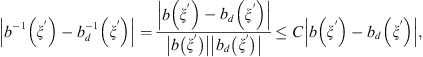 because
  then we will estimate the latter difference. Simplest considerations lead to the following estimate,

We will estimate one integral only, the second one is almost the same,

Therefore if  is a bounded function we have the required estimate.
Conclusion
This paper is one of first steps for studying discrete boundary value problems and their connections with classical theory of boundary value problems for elliptic pseudo-differential equations. We intend to study more general situations in forthcoming papers and to obtain approximation estimates for comparison of discrete and continuous solutions.
Acknowledgments
Research supported by the State contract of the Russian Ministry of Education and Science (contract No 1.7311.2017/8.9).
References
- Eskin GI (1981), Boundary value problems for elliptic pseudodifferential equations, AMS, Providence. [Google Scholar]
- Taylor ME (1980), Pseudo-differential operators, Princeton Univ. Press, Princeton. [Google Scholar]
- Vasil’ev AV, Vasil’ev VB (2015), Periodic Riemann problem and discrete convolution equations. Diff Equ 51, 5, 652–660. [CrossRef] [Google Scholar]
- Vasilyev AV, Vasilyev VB (2015), Discrete singular integrals in a half-space. Current trends in analysis and its applications, Proc. 9th ISAAC Congress, Kraków, Poland, Birkhäuser, Basel, pp. 663–670. [Google Scholar]
- Vasilyev AV, Vasilyev VB (2017), Two-scale estimates for special finite discrete operators. Math Model Anal 22, 3, 300–310. [CrossRef] [Google Scholar]
- Samarskii AA (2001), The theory of difference schemes, CRC Press, Boca Raton. [CrossRef] [Google Scholar]
- Vasilyev AV, Vasilyev VB (2018), Pseudo-differential operators and equations in a discrete half-space. Math Model Anal 23, 3, 492–506. [CrossRef] [Google Scholar]
- Vasilyev AV, Vasilyev VB (2018), On some discrete boundary value problems in canonical domains, in: Differential and Difference Equations and Applications. Springer Proc. Math. Stat, Vol. 230, Springer, Cham, pp. 569–579. [CrossRef] [Google Scholar]
- Ryaben’kii VS (2002), Method of difference potentials and its applications, Springer-Verlag, Berlin-Heidelberg. [CrossRef] [Google Scholar]
- Vasilyev VB (2017), Discreteness, periodicity, holomorphy, and factorization, in: C Constanda, M Dalla Riva, PD Lamberti, P Musolino (Eds.), Integral Methods in Science and Engineering, Theoretical Technique, Vol. 1. Birkhauser, Cham, Switzerland, pp. 315–324. [CrossRef] [Google Scholar]
- Vasilyev AV, Vasilyev VB (2016), Difference and discrete equations on a half-axis and the Wiener-Hopf method. Azerb J Math 6, 1, 79–86. [Google Scholar]
- Vasilyev AV, Vasilyev VB (2016), On solvability of some difference-discrete equations. Opusc Math 36, 4, 525–539. [CrossRef] [Google Scholar]
- Vasilyev AV, Vasilyev VB (2016), On finite discrete operators and equations. Proc Appl Math Mech 16, 1, 771–772. [Google Scholar]
- Vasilyev VB (2017), The periodic Cauchy kernel, the periodic Bochner kernel, and discrete pseudo-differential operators. AIP Conf Proc 1863, 140014-1–140014-4. [Google Scholar]
- Vasilyev VB (2018), Discrete pseudo-differential operators and boundary value problems in a half-space and a cone. Lobachevskii J Math 39, 2, 289–296. [CrossRef] [Google Scholar]
- Vasilyev VB (2018), On discrete pseudo-differential operators and equations. Filomat 32, 3, 975–984. [CrossRef] [Google Scholar]
- Vasilyev VB (2018), On some approximate calculations for certain pseudo-differential equations. Bull Karaganda Univ Math 3, 91, 9–16. [CrossRef] [Google Scholar]
Cite this article as: Tarasova O.A & Vasilyev V.B 2019. To the theory of discrete boundary value problems. 4open, 2, 17.