© V.A. González-López et al., Published by EDP Sciences, 2019

1 Introduction

The research based on copula models offers flexibility to represent multivariate structures, since the use of Sklar’s theorem [1] allows us to split the problem of determining the multivariate structure in two stages, (a) with focus on the univariate marginal distributions and (b) with focus on the dependence structure, properly speaking, the copula function. This approach can be very attractive if stage (a) is simplified by characteristics of the real problem. In this paper we point to this situation, since the observed values are relevant in relation to the positions they take in the sample (their ranks). The models of copula allow to incorporate to the study a great diversity of types of dependence. Despite the enormous flexibility offered by the copulas they are not free from the limitations imposed by small or moderate data sets and, for such situations, alternative approaches make sense, such as adopting a Bayesian perspective or a non-parametric perspective based on, for instance, the ranks of the observations. In this paper, we conduct a trivariate dependence study and our focus is to inspect conditional probabilities estimated by the copula. More precisely, our object of inspection are probabilities in the tails, close to the extreme values, for which copulas are especially useful. The copula has a domain given by the cartesian product of several intervals [0, 1], it scales the observed values to this domain and thus, transforms the extreme values of the original observations into values close to 0 and 1. We base the trivariate study on a type of copula with bivariate and non-negative Spearman’s coefficients. From the bivariate and uniparametric model introduced in [2] (family 2.8) using the mixture representation (theorem 4.6.2 in [3]) we extend the model to the trivariate case. With these tools we inspect data from students of the University of Campinas, all of them selected for the undergraduate course of Statistics, with entrance in 2013, 2014 and 2015 respectively. The database is composed by two scores related to the section of the entrance exam that evaluates exact sciences. The dataset also records the scores obtained by these students in Calculus I (subject of the first period in the course). In this paper, we create a representation for the predictive power that the specific topics of the entrance exam have as to predict the performance in Calculus I. That is, we model and compare the 3 years looking for subsidies that allow us to answer if there has been an improvement in the predictive capacity of those topics of the entrance exam, as the years go by. This question is especially relevant from 2014 to 2015, when happened a revision of the topics evaluated by the entrance exam.

In Section 2, we discuss the preliminary concepts to deal with trivariate analysis, as is the case. In Section 3, we introduce the problem and perform an inspection of the database. In Section 4, we introduce the model to be estimated and the connection with the tail probabilities that we will estimate. Also, in Section 4, we introduce the estimators of those probabilities. The general conclusions are given in Section 5.

2 Preliminaries

Given a pair of random variables (X ₁, X ₂) with cumulative 2-distribution H and marginal distributions F _i , i = 1, 2, i.e. ∀x, F ₁ (x) = H(x,∞) and F ₂ (x) = H(∞, x), there exists a cumulative distribution C:[0, 1]²→[0, 1] with Uniform marginal distributions $\left(C\right(u,1)=u, C(1,u)=u, \forall u\in [\mathrm{0,1}\left]\right)$ such that, $\forall (x_1,x_2)$ value of (X ₁, X ₂),

$$H(x_1,x_2)=C\left(F_1\right(x_1),F_2(x_2\left)\right).$$(1)

Then, C is the 2-copula of (X ₁, X ₂), see [1]. If X ₁ and X ₂ are continuous the 2-copula is unique, otherwise, C is uniquely determined on the product of ranges Ran F ₁ × Ran F ₂. This result can be extended for any dimension greater than 2. C represents the dependence between the variables X ₁ and X ₂. That is, being H the joint distribution between X ₁ and X ₂, where H results from the composition between C, F ₁ and F ₂ (see Eq. (1)) while F _i exposes the marginal law of X _i (which is not related to X _j , i ≠ j) C quantifies the relationship between X ₁ and X ₂. Moreover, it also quantifies the dependence between the variables F ₁ (X ₁) and F ₂ (X ₂). As we shall see, dependence coefficients show the copula in its analytical form. Given a pair (X ₁, X ₂) of continuous random variables with associated 2-copula C, the population version ρ ₁₂ (C) of Spearman’s rho, is ${\rho }_{12}\left(C\right)=12{\int }_{I^2}\mathrm{}C(u,v)\mathrm{d}u\mathrm{d}v-3,$ where I = [0, 1]. In the trivariate case, where (X ₁, X ₂, X ₃) is a vector of continuous random variables with 3-copula C, there are several generalizations of Spearman’s rho. They are, (a) the average of the three pairwise measures ρ ₁₂, ρ ₁₃ and ρ ₂₃, ${\rho }_3^{\mathrm{*}}\left(C\right)=\frac{{\rho }_{12}+{\rho }_{13}+{\rho }_{23}}{3},$ (b) the trivariate generalizations ${\rho }_3^{-}\left(C\right)=8{\int }_{I^3}\mathrm{}C(u,v,w)\mathrm{d}u\mathrm{d}v\mathrm{d}w-1,$ ${\rho }_3^{+}\left(C\right)=8{\int }_{I^3}\mathrm{}\bar{C}\left(u,v,w\right) \mathrm{d}u\mathrm{d}v\mathrm{d}w-1,$ where $\bar{C}$ denotes the survival function associated with C, and (c) the coefficients of directional dependence ${\rho }_3^{({\alpha }_1,{\alpha }_2,{\alpha }_3)}\left(C\right)$ introduced by [4], where ${\alpha }_i\in \left\{-\mathrm{1,1}\right\},$ given by ${\rho }_3^{({\alpha }_1,{\alpha }_2,{\alpha }_3)}\left(C\right)=8{\int }_{I^3}\mathrm{}{Q}_{{\alpha }_1,{\alpha }_2,{\alpha }_3}(u,v,w)$ dudvdw, where $Q_{{\alpha }_1,{\alpha }_2,{\alpha }_3}(u,v,w)= \mathrm{Prob} ({\alpha }_1{X}_1>{\alpha }_{1}u,{\alpha }_2{X}_2>{\alpha }_{2}v,{\alpha }_3{X}_3>{\alpha }_{3}w)- \mathrm{Prob} ({\alpha }_1{X}_1>{\alpha }_{1}u) \mathrm{Prob} ({\alpha }_2{X}_2>{\alpha }_{2}v) \mathrm{Prob} ({\alpha }_3{X}_3>{\alpha }_{3}w).$ According to [4], ${\rho }_3^{({\alpha }_1,{\alpha }_2,{\alpha }_3)}\left(C\right)$ is a linear combination of the pairwise measures and the measures ${\rho }_3^{+}$ and ${\rho }_3^{-},$ given by ${\rho }_3^{({\alpha }_1,{\alpha }_2,{\alpha }_3)}=\frac{{\alpha }_1{\alpha }_2{\rho }_{12}+{\alpha }_1{\alpha }_3{\rho }_{13}+{\alpha }_2{\alpha }_3{\rho }_{23}}{3}+{\alpha }_1{\alpha }_2{\alpha }_3\frac{({\rho }_3^{+}-{\rho }_3^{-})}{2}.$ Equivalently, ${\rho }_3^{({\alpha }_1,{\alpha }_2,{\alpha }_3)}\left(C\right)$ is equal to ${\rho }_3^{+}\left(C^{\text{'}}\right),$ where $C^{\text{'}}$ is the copula associated with the random variables (α ₁ X ₁, α ₂ X ₂, α ₃ X ₃). The purpose of the directional ρ-coefficients ${\rho }_3^{({\alpha }_1,{\alpha }_2,{\alpha }_3)}$ is to detect positive dependence among the random variables X ₁, X ₂, X ₃ undetected by the coefficients ${\rho }_3^{\mathrm{*}},{\rho }_3^{+}$ and ${\rho }_3^{-}.$ Also note that ${\rho }_3^{(\mathrm{1,1},1)}={\rho }_3^{+}$ and ${\rho }_3^{(-1,-1,-1)}={\rho }_3^{-}.$ García Jesús et al. [5] proposes to study the following index, with the objective of identifying the highest positive trivariate correlation, among all the possible directions, ${\rho }_3^{ \max }\left(C\right)={\max }_{({\alpha }_1,{\alpha }_2,{\alpha }_3)}\left\{{\rho }_3^{({\alpha }_1,{\alpha }_2,{\alpha }_3)}\left(C\right)\right\}.$ In [5], is proved that ${\rho }_3^{ \max }=\frac{2}{3}\max \left\{{\rho }_{12},{\rho }_{13},{\rho }_{23},3{\rho }_3^{\mathrm{*}}\right\}-\min \left\{{\rho }_3^{+},{\rho }_3^{-}\right\}.$ Suppose that the maximum ${\rho }_3^{ \max }$ is reached in the direction (−1, −1, 1), this means that the maximum correlation has been given between events type $\{X_1\le u\},\{X_2\le v\}$ and $\{X_3>w\}.$ Table 1 shows how to determine the direction which produces the maximal value of ${\rho }_3^{({\alpha }_1,{\alpha }_2,{\alpha }_3)}.$

Nelsen et al. [4] and García Jesús et al. [5] expose various situations where the coefficients of directional dependence ${\rho }_3^{\alpha }$ and consequently the index ${\rho }_3^{ \max }$ are able to capture positive dependence not detected by the traditional 3-variate coefficients ${\rho }_3^{\mathrm{*}}, {\rho }_3^{+}$ and ${\rho }_3^{-}.$ Also, in the next subsection we will give an example in which is evident the usefulness of the coefficients of directional dependence.

All these coefficients are estimated from the ranks of the observations, as we will see below.

2.1 Estimation of coefficients

Consider a trivariate random sample ${\left\{(X_{1j},X_{2j},X_{3j})\right\}}_{j=1}^n$ of the vector (X ₁, X ₂, X ₃) with associated unknown copula C. Let be R _ij  = rank of X _ij in $\left\{X_{i1},\dots ,X_{\mathrm{in}}\right\}$ and define ${\bar{R}}_{\mathrm{ij}}=n+1-R_{\mathrm{ij}},$ for i = 1, 2, 3. The nonparametric estimators are ${\widehat{\rho }}_{\mathrm{ik}}=\frac{12}{n(n^2-1)}{\sum }_{\mathrm{j}=1}^n\mathrm{}{R}_{\mathrm{ij}}{R}_{\mathrm{kj}}-3\frac{(n+1)}{(n-1)}, \mathrm{ik}\in \left\{12, 23, 13\right\}, {\widehat{\rho }}_3^{-}=\frac{8}{n(n-1)(n+1{)}^2}{\sum }_{j=1}^n\mathrm{}{R}_{1j}{R}_{2j}{R}_{3j}-\frac{(n+1)}{(n-1)},$ ${\widehat{\rho }}_3^{+}=\frac{8}{n(n-1)(n+1{)}^2}{\sum }_{j=1}^n\mathrm{}{\bar{R}}_{1j}{\bar{R}}_{2j}{\bar{R}}_{3j}-\frac{(n+1)}{(n-1)}.$ Set $R_{\mathrm{ij}}^{{\alpha }_i}$ to be R _ij if α _i  = −1 and ${\bar{R}}_{\mathrm{ij}}$ if α _i  = 1, and define the estimator of the coefficient of directional dependence ${\widehat{\rho }}_3^{({\alpha }_1,{\alpha }_2,{\alpha }_3)}=\frac{8}{n(n-1)(n+1{)}^2}{\sum }_{j=1}^n\mathrm{}{R}_{1j}^{{\alpha }_1}{R}_{2j}^{{\alpha }_2}{R}_{3j}^{{\alpha }_3}-\frac{(n+1)}{(n-1)}.$ The plug-in estimator of ${\rho }_3^{ \max }$ is given by ${\widehat{\rho }}_3^{ \max }=\frac{2}{3}\max \left\{{\widehat{\rho }}_{12},{\widehat{\rho }}_{13},{\widehat{\rho }}_{23},3{\widehat{\rho }}_3^{\mathrm{*}}\right\}-\min \left\{{\widehat{\rho }}_3^{+},{\widehat{\rho }}_3^{-}\right\},$ where $3{\widehat{\rho }}_3^{\mathrm{*}}={\widehat{\rho }}_{12}+{\widehat{\rho }}_{13}+{\widehat{\rho }}_{23}.$

In the following example we show how the directional ρ coefficients summarize in one number the dependence behavior in a trivariate random vector. For instance, between two variables we can observe concordance (both growing) or discordance (one growing and the other not) and in the trivariate case we can have combinations of those situations.

Example 2.1

The data is coming from [6], it is part of the dataset Intercountry Life-Cycle Savings Data which are averaged over the decade 1960–1970. It is composed by n = 50 observations of two demographic variables (i) the percentage of population less than 15 years old and (ii) the percentage of the population over 75 years old and one economic variable (iii) the per-capita disposable income, coming from the countries: Australia, Austria, Belgium, Bolivia, Brazil, Canada, Chile, China, Colombia, Costa Rica, Denmark, Ecuador, Finland, France, Germany, Greece, Guatamala, Honduras, Iceland, India, Ireland, Italy, Japan, Korea, Luxembourg, Malta, Norway, Netherlands, New Zealand, Nicaragua, Panama, Paraguay, Peru, Philippines, Portugal, South Africa, South Rhodesia, Spain, Sweden, Switzerland, Turkey, Tunisia, United Kingdom, United States, Venezuela, Zambia, Jamaica, Uruguay, Libya, Malaysia.

In Table 2 , we report all the coefficient’s estimates. We see that ${\widehat{\rho }}_3^{\max }=0.84157$ exposes a positive and marked value. Note, on the other hand, that none of the traditional trivariate coefficients ${\widehat{\rho }}_3^{-},$ ${\widehat{\rho }}_3^{+}$ or ${\widehat{\rho }}_3^{*}$ detect positive dependence. Even more, only one of the pair coefficients ( ${\widehat{\rho }}_{23}=0.80723$ ) shows a positive value, as is evident from the inspection of Figure 2a . In Figure 2b , the scale of colors goes from red to black when the values in the axis “pop75” grows. In red the smaller values and in black the highest ones, going through a red-black color. This attribute is exercised by the option “highlight.3d” of the function “scatterplot3d” from the “Scatterplot3d” package of R-project.

Table 3 shows in which situation this data is found, among those detailed in Table 1 . We see that the variables pop75 and dpi are concordant, in the sense shown in Figure 2a , while each one of them is discordant with pop15, as seen in Figure 1 . Thus, it is expected that the maximum dependence occurs in α = (1, −1, −1) and α = (−1, 1, 1). In Figure 3 , we show the scatterplots between the margial ranks of the three original variables (on (a)) and those variables oriented in the direction of the maximal dependence (1, −1, −1) (on (b)). Note that this means that ${\rho }_3^{\max }(\mathrm{pop}15, \mathrm{pop}75, \mathrm{dpi})={\rho }_3^{+}(\mathrm{pop}15,-\mathrm{pop}75,-\mathrm{dpi}).$

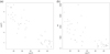Figure 1 (a) Percentage of population less than 15 years old (pop15) vs. percentage of the population over 75 years old (pop75). (b) Percentage of population less than 15 years old (pop15) vs. per-capita disposable income (dpi). Observations of n = 50 countries (see [6]).

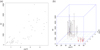Figure 2 (a) Percentage of the population over 75 years old (pop75) vs. per-capita disposable income (dpi). (b) Scatterplot between pop15, pop75 and dpi, from red to black color in increasing order in relation to the “pop75” axis. Observations of n = 50 countries (see [6]).

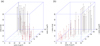Figure 3 (a) Scatterplot between ranks of pop15, ranks of pop 75 and ranks of dpi, from red to black color in increasing order in relation to the “ranks of pop75” axis. (b) Scatterplot between ranks of pop15, – ranks of pop 75 and – ranks of dpi, since ${\rho }_3^{\max }(\mathrm{pop}15,\mathrm{pop}75,\mathrm{dpi})={\rho }_3^{+}(\mathrm{pop}15,-\mathrm{pop}75,-\mathrm{dpi}).$ From red to black color in increasing order in relation to the “– ranks of pop75” axis.

In this way, the maximum trivariate dependence occurs in events of type: $\{ \mathrm{ranks} \mathrm{of} \mathrm{pop}15 >u\},\{ \mathrm{ranks} \mathrm{of} \mathrm{pop}75 \le v\},\{ \mathrm{ranks} \mathrm{of} \mathrm{dpi}\le w\}.$

In some situations like the one investigated in this work, given the meaning of the variables, it is expected that the maximal dependence will hold a specific behavior, occurring in certain directions, and the maximal dependence index ${\rho }_3^{ \max }$ allows to verify whether this actually happens or not. For example, if a whole concordance is expected, in all variables of the vector, the maximum dependence must occur in the directions (1, 1, 1) and/or (−1, −1, −1), corresponding with a maximal dependence detected by the coefficients ${\rho }_3^{+}$ and/or ${\rho }_3^{-}$.

3 Assessment of recruitment system

The University of Campinas (Unicamp) is one of the three most recognized public universities in the state of São Paulo in Brazil, these are: Unesp (São Paulo State University), Unicamp and USP (University of São Paulo). Unicamp is responsible for about 15% of the country’s scientific production, offering graduate courses, undergraduate courses and technical high schools courses. The institution offers about 70 undergraduate courses in the most diverse areas of knowledge, each course offers a specific number of places per year. Candidates are selected through an evaluation process in different areas of knowledge and certain subjects are more relevant than others to achieve the necessary score for the admission in a specific course. This is the case of the Statistics undergraduate course inserted in the exact sciences. The entrance exam during the period 2013–2015 was composed of a first phase of various general knowledge areas and two writings. And a second phase constituted in 2013 and 2014 by specific tests in (i) Writing (ii) Mathematics, (iii) Portuguese, (iv) Humanities and Arts, (v) English and (vi) Natural Sciences. In 2015, (iv) and (vi) were split in (a) Physics, (b) Biology, (c) Chemistry, (d) History and (e) Geography. For the undergraduate course of Statistics the most relevant disciplines in the 2013–2014 versions are: Mathematics and Natural Sciences and for 2015, Mathematics and Physics. An assumption that is used as the basis for the conception of the entrance exams in this format is that certain subjects of the entrance exam could measure the ability of a student in relation to some subjects of the course. For example, a student of the undergraduate course of Statistics should take lessons of calculus, analysis, algebra, etc, and in that case mathematics and natural sciences (or physics), of the entrance exam, would be potential predictors of performance in those subjects. And that may be one of the reasons why the entrance exam has been modified from 2014 to 2015.

In this paper, we implement a trivariate study that involves the Calculus I subject of the undergraduate course in Statistics (taken at the begin of the course) and two subjects of the entrance exam: for 2013 and 2014 (1) Mathematics and (2) Natural Sciences and for 2015 (1) Mathematics and (2) Physics. We wish to estimate the probability that, given a poor performance in (1) and (2), a poor performance occurs in Calculus I, and we also want to estimate the probability that, given an efficient performance in (1) and (2), the performance in Calculus I be efficient. We would also like to evaluate if the alteration occurred from 2014 to 2015 in the entrance examination caused positive modifications in this regard. That is, we expect an increase in such probabilities.

3.1 Data set

The database is composed of annual trivariate data of students of the undergraduate course in Statistics at Unicamp, corresponding to three consecutive years: 2013, 2014 and 2015 and involving two subjects of the entrance examination of Unicamp and the subject of Calculus I, the latter already being studied during the course in Statistics at Unicamp. We have considered the two most related subjects with exact sciences and that made part of the group of subjects evaluated in the entrance examination, in 2013 and 2014 these are: Mathematics and Natural Sciences. Already for 2015, the entrance exam was modified, and the two subjects most related to Calculus I are: Mathematics and Physics, see Figures 4–6. In this paper, the Calculus I grades are identified with the variable X ₁ , the Mathematics (of the entrance exam) with X ₂ and depending on the year, X ₃ represents Natural Sciences or Physics.

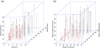Figure 4 Data of 2013. (a) Scatterplot between Calculus I, Mathematics and Natural Sciences, from red to black color in increasing order in relation to the “Mathematics” axis. (b) Scatterplot between ranks of Calculus I, ranks of Mathematics and ranks of Natural Sciences, from red to black color in increasing order in relation to the “Ranks of Mathematics” axis.

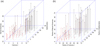Figure 5 Data of 2014. (a) Scatterplot between Calculus I, Mathematics and Natural Sciences, from red to black color in increasing order in relation to the “Mathematics” axis. (b) Scatterplot between ranks of Calculus I, ranks of Mathematics and ranks of Natural Sciences, from red to black color in increasing order in relation to the “Ranks of Mathematics” axis.

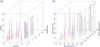Figure 6 Data of 2015. (a) Scatterplot between Calculus I, Mathematics and Physics, from red to black color in increasing order in relation to the “Mathematics” axis. (b) Scatterplot between ranks of Calculus I, ranks of Mathematics and ranks of Physics, from red to black color in increasing order in relation to the “Ranks of Mathematics” axis.

We see, from Table 5, that the directions of maximal dependence follow the expected trend. That is, we expect a greater concentration of the dependence in the directions (1, 1, 1) and (−1, −1, −1) which would indicate that large $\{X_1>u,X_2>v,X_3>w\}$ or low $\{X_1\le u,X_2\le v,X_3\le \mathrm{w}\}$ grades capture the highest correlation.

In 2013 and 2015 the maximum dependence occurs in the direction (−1, −1, −1), while in 2014 the maximum dependence occurs in the direction (1, 1, 1). For each year the magnitude of the directional dependencies ${\rho }_3^{+}$ and ${\rho }_3^{-}$ is similar. Remarkable is the low and maximal 3-variate directional correlation (${\widehat{\rho }}_3^{-}=0.45749$) observed in 2013.

To compute the probabilities that we want, we will take into account the dependence between the three variables. For such we appeal to the notion of copula that will allow us to model this dependence.

4 Dependence and tail probabilities

Returning to the context of equation (1) in the trivariate case, we define (U ₁, U ₂, U ₃) := (F ₁ (X ₁),F ₂ (X ₂),F ₃ (X ₃)) that is, that each variable X _i is transformed into F _i (X _i ). Given that F _i is the cumulative distribution of X _i , X _i is subjected to a non-decreasing monotonic transformation. Each marginal F _i rescales X _i to [0, 1] which allows inserting the three variables in the same spectrum of variability. The joint distribution between U ₁, U ₂ and U ₃ is the copula referenced in equation (1). Our purpose to follow is to formulate an adequate construction of C for (U ₁, U ₂, U ₃), which will lead us to adopt the trivariate Joe’s copula in data modeling.

As we have already observed, the Spearman’s rho coefficientes in the current study assume positive values, which leads us to consider models that respect this condition. One of the bivariate models of considerable flexibility and easy interpretation is that given by the copula introduced in [2] (bivariate Joe’s copula), whose properties are widely investigated in [2] and [3]. The most striking property is that as the Spearman’s rho coefficiente increases, the value of the parameter that indexes the bivariate model also increases, and vice versa. The bivariate version covers from the independence case (C(u,v) = uv) to the extreme positive dependence case ($C(u,v)=\min \{u,v\}$). The copula model presented below is a generalization of [2] and will be formulated by means of an Archimedean generator. The bivariate family is

$$C(u,v|\delta )=1-\{{\bar{u}}^{\delta }+{\bar{v}}^{\delta }-{\bar{u}}^{\delta }{\bar{v}}^{\delta }{\}}^{\frac{1}{\delta }}, 1\le \delta <\infty , \bar{u}=1-u,\bar{v}=1-v, u,v\in \left[\mathrm{0,1}\right].$$(2)

A simple way to extend this model to dimension 3 is by considering the fact that (2) is an Arquimedian copula, and therefore can be constructed from an Arquimedian generator. That is, in the case of the model (2) the generator is $\varphi \left(t\right)=-\ln (1-[1-t{]}^{\delta }), \delta \in [1,\mathrm{\infty })$ then, $C(u,v|\delta )={\varphi }^{-1}(\varphi \left(u\right)+\varphi \left(v\right))$ with ${\varphi }^{-1}\left(s\right)=1-[1-e^{-s}{]}^{\frac{1}{\delta }}.$ Since ϕ is a continuous strictly decreasing function from [0, 1] to [0, ∞] such that ϕ(0)=∞ and ϕ(1) = 0,

$$\begin{array}{cc}C(u,v,w|\delta )={\varphi }^{-1}(\varphi \left(u\right)+\varphi \left(v\right)+\varphi \left(w\right)), & u,v,w\in \left[\mathrm{0,1}\right]\end{array}$$(3)is also a copula (see Thm. 4.6.2 in [3]). Naturally this way of constructing copulas can be extended to dimensions greater than 3. Note that the bivariate marginal cumulatives derived from (3) are bivariate copulas type (2), for instance $C(u,v,1|\delta )$ of equation (3) is equal to $C(u,v|\delta )$ of equation (2). So, the 3-copula is given by

$$C(u,v,w|\delta )=1-\{1-\left(1-{\bar{u}}^{\delta }\right)\left(1-{\bar{v}}^{\delta }\right)\left(1-{\bar{w}}^{\delta }\right){\}}^{\frac{1}{\delta }}, \bar{u}=1-u,\bar{v}=1-v,\bar{w}=1-w, u,v,w\in \left[\mathrm{0,1}\right].$$

As the annual database is compound by around 60 observations (see Tab. 4), it seems reasonable to maintain only one parameter δ in the formulation of the model. $C(u,v,w|\delta =1)=\mathrm{uvw}$ is the 3-copula of independence and when the value of δ is near to one, strongest is the evidence of joint independence, between the variables. The estimation of the parameter of the copula allows the construction of conditional probabilities which make possible the inspection of the dependence’s impact in the tail probability year after year. More precisely, if we want to estimate $\mathrm{Prob} (U_1\le u|U_2\le v,U_3\le w)$ and $\mathrm{Prob} (U_1>u|U_2>v,U_3>w),$ we can use the following relationships:

$$\begin{array}{cc}\mathrm{Prob} (U_1\le u|U_2\le v,U_3\le w)& =\frac{ \mathrm{Prob} (U_1\le u,U_2\le v,U_3\le w)}{ \mathrm{Prob} (U_2\le v,U_3\le w)}\\ & =\frac{C(u,v,w)}{C(1,v,w)}.\end{array}$$(4)

Since,

$$\begin{array}{cc}\mathrm{Prob} (U_2>v,U_3>w)& =1- \mathrm{Prob} (U_2\le v)- \mathrm{Prob} (U_3\le w)+ \mathrm{Prob} (U_2\le v,U_3\le w)\\ & =1-v-w+C(1,v,w),\end{array}$$(5)and

$$\begin{array}{cc}\mathrm{Prob} (U_1>u,U_2>v,U_3>w)& = \mathrm{Prob} (U_1>u)- \mathrm{Prob} (U_1>u,U_2\le v)- \mathrm{Prob} (U_1>u,U_3\le w)+ \mathrm{Prob} (U_1>u,U_2\le v,U_3\le w)\\ & =1-u-[ \mathrm{Prob} (U_2\le v)- \mathrm{Prob} (U_1\le u,U_2\le v\left)\right]-[ \mathrm{Prob} (U_3\le w)- \mathrm{Prob} (U_1\le u,U_3\le w\left)\right]+[ \mathrm{Prob} (U_2\le v,U_3\le w)- \mathrm{Prob} (U_1\le u,U_2\le v,U_3\le w\left)\right]\\ & =1-u-v-w+C(u,v,1)+C(u,1,w)+C(1,v,w)-C(u,v,w),\end{array}$$(6)from (5) and (6), we obtain

$$\begin{array}{cc}\mathrm{Prob} (U_1>u|U_2>v,U_3>w)& =\frac{ \mathrm{Prob} (U_1>u,U_2>v,U_3>w)}{ \mathrm{Prob} (U_2>v,U_3>w)}\\ & =\frac{1-u-v-w+C\left(u,v,1\right)+C\left(u,1,w\right)+C\left(1,v,w\right)-C\left(u,\mathrm{v},w\right)}{1-v-w+C\left(1,v,w\right)}.\end{array}$$(7)

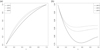
In Figure 7 we see the trend of the conditional probabilities (4) and (7), for Joe’s model (Eq. (3)). In both cases as the δ value increases so do the conditional probabilities. This characteristic is related to the connection between the δ parameter and the Spearman’s rho coefficient, which grows as δ grows. For instance, $C(u,v,1|1)=\mathrm{uv}$ (corresponding to ρ ₁₂=0) and, when δ grows $C(u,v,1,|\delta )$ tends to $\min \{u,v\}$ (corresponding to ρ ₁₂ = 1). Equivalently it happens for the other combinations of variables two to two, of U ₁, U ₂ and U ₃.

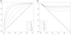Figure 7 (a) $\mathrm{Prob} (U_1\le u|U_2\le u,U_3\le u)$ from equations (3) to (4), with δ = 1, 2, 4, 10, 20. (b) $\mathrm{Prob} (U_1>u|U_2>u,U_3>u)$ from equations (3) to (7), with δ = 1, 1.5, 2, 2.5, 3.

We note that the quantities (4) and (7) (for values close to u = v = w = 0 and u = v = w = 1, respectively) are the ones that should grow from 2013 to 2015, according to what is expected, if there has been an increase in the predictive capacity of the entrance exam. Proximity to zero refers to low grades and poor performance and proximity to one refers to high grades and efficient performance.

Setting an interval for U ₂ and U ₃, let’s say [a, b], we can compute the probability of U ₁ being less than or equal to u. This computation allows us to quantify the effect of U ₂ and U ₃ on U ₁. So,

$$\mathrm{Prob} (U_1\le u|U_2\in [a,b],U_3\in [a,b])=\frac{C(u,b,b)+C(u,a,a)-C(u,a,b)-C(u,b,a)}{C(1,b,b)+C(1,a,a)-C(1,a,b)-C(1,b,a)}$$(8)and in a complementary way

$$\mathrm{Prob} (U_1>u|U_2\in [a,b],U_3\in [a,b])=1- \mathrm{Prob} (U_1\le u|U_2\in [a,b],U_3\in [a,b\left]\right).$$(9)

An inspection of this quantities could provide an estimate of the expected range of the conditional probability, given an interval [a, b] and a threshold of interest u.

4.1 Estimation

In this section we discuss the estimation process. The values observed annually $\left\{\right(X_{1,j},X_{2,j},X_{3,j}){\}}_{j=1}^n$ will be transformed by their marginal ranks re-scaled to [0, 1], with n given by Table 4, year by year. In this way, the triples ${\left\{\left(\frac{R_{1,j}}{n},\frac{R_{2,j}}{n},\frac{R_{3,j}}{n}\right)\right\}}_{j=1}^n$ represent the values of (U ₁, U ₂, U ₃). Then, U ₁ are the ranks of the grades in Calculus I scaled to [0, 1], U ₂ are the ranks of the grades of Mathematics scaled to [0, 1] and U ₃ are the ranks of the grades of Natural Sciences (2013–2014) or Physics (2015) scaled to [0, 1]. Note also that working with ranks turn the data comparable, even though the entrance exam applied is different each year.

From equation (3), it is possible to derive the density of the copula, say $c(u,v,w|\delta ),$ and to implement the process of estimating the parameter (δ). In the present case we give space to a Bayesian procedure, since the annual database shows a moderate size (Tab. 4). We assume a non-informative priori distribution on δ, that is, π(δ) ∝ k (constant value), then the posteriori distribution of δ is proportional to the likelihood.

$$\prod _{i=1}^n\mathrm{}c\left(\frac{R_{1,j}}{n},\frac{R_{2,j}}{n},\frac{R_{3,j}}{n}|\delta \right).$$(10)

Under quadratic loss function, the Bayesian estimator is the mean of the posterior distribution of δ, and this will be the estimator ${\widehat{\delta }}_B,$ obtained by Importance Sampling (see [7]). For comparison we have also registered the frequentist estimators, we adopted the semiparametric method suggested in [8]. Thus, ${\widehat{\delta }}_F$ denotes the estimates obtained by maximization of the pseudo-loglikelihood, given by equation (11)

$$\sum _{i=1}^n\mathrm{}\ln \left[c\left(\frac{R_{1,j}}{n},\frac{R_{2,j}}{n},\frac{R_{3,j}}{n}|\delta \right)\right].$$(11)

The classical estimators ${\widehat{\delta }}_F$ were obtained by the function fitCopula (method mpl) available in the R package Copula from R project for Statistical Computing (see https://cran.r-project.org/web/packages/copula/copula.pdf). ${\widehat{\delta }}_B$ is the Bayesian estimator of the expected value,

$${\delta }^{\mathrm{*}}={\mathbb{E}}_{\pi (·|\mathrm{Data})}\left(\delta \right)={\int }_1^{\mathrm{\infty }}\mathrm{}\delta \pi \left(\delta \right|\mathrm{Data})\mathrm{d}\delta ,$$(12)where $\pi \left(\delta \right|\mathrm{Data})$ is the posterior density of δ and δ ≥ 1. By Importance Sampling and knowing the posterior density $\pi (·|\mathrm{Data})$ we choose a density q(·) from what is easy to generate values of δ, say δ ₁, …, δ _m and we can define the approximation of equation (12) by,

$$\widehat{\delta }=\frac{1}{m}\sum _{i=1}^m\mathrm{}{\delta }_{i}w\left({\delta }_i\right),$$with $w\left(\delta \right)=\frac{\pi \left(\delta \right|\mathrm{Data})}{q\left(\delta \right)}.$ Since, under regularity conditions ${\delta }^{\mathrm{*}}={\mathbb{E}}_{q(·)}\left(\delta w\right(\delta \left)\right).$ In the present situation we only can access to a function that is proportional to $\pi (·|\mathrm{Data}),$ which is given by equation (10) and $\pi \left(\delta \right|\mathrm{Data})=c_o{\prod }_{i=1}^n\mathrm{}c\left(\frac{R_{1,j}}{n},\frac{R_{2,j}}{n},\frac{R_{3,j}}{n}|\delta \right)$ for an unknown contant c _o . In that case, the self-normalized Importance Sampling estimator of δ ^* is given by,

$${\widehat{\delta }}_B=\frac{\frac{1}{m}\sum _{i=1}^m\mathrm{}{\delta }_i{w}^{\mathrm{\prime }}\left({\delta }_i\right)}{\frac{1}{m}\sum _{i=1}^m\mathrm{}{w}^{\mathrm{\prime }}\left({\delta }_i\right)},\hspace{0.5em}\mathrm{with}\hspace{0.5em}{w}^{\mathrm{\prime }}\left(\delta \right)=\frac{\prod _{i=1}^n\mathrm{}c\left(\frac{R_{1,j}}{n},\frac{R_{2,j}}{n},\frac{R_{3,j}}{n}|\delta \right)}{q\left(\delta \right)},$$(13)and ${\widehat{\delta }}_B=\frac{\frac{1}{m}{\sum }_{i=1}^m\mathrm{}{\delta }_{i}w\left({\delta }_i\right)}{\frac{1}{m}{\sum }_{i=1}^m\mathrm{}w\left({\delta }_i\right)}.$ In this case we use as q(·) an exponential density of rate 1 and properly accommodated in the support [1,∞). This function looks appropriate since it attributes zero density to δ < 1. For a description of the quality of the Bayesian estimator (13) see Table 7, where we expose (a) the mean of 1000 replicates of equation (13) and (b) the standard deviation of (a).

We see that up to the second decimal position in Table 6 the estimates are consistent with the means in Table 7 (a), reflecting the standard deviation, reported in Table 7 (b).

We note that the value of $\widehat{\delta }$ in both versions (${\widehat{\delta }}_F$ and ${\widehat{\delta }}_B$) grows from 2013 to 2015, showing that the dependence between (U ₁, U ₂, U ₃) grows year by year. This is positive evidence that will have an impact on the conditional probabilities. Using any estimator $\widehat{\delta }$ we can define estimations for any operation involving the copula. For instance, following the functional forms of equations (4), (8), (9) and (7), we define

$$\widehat{\mathrm{Prob}}(U_1\le u|U_2\in [a,b],U_3\in [a,b])=\frac{C(u,b,b|\widehat{\delta })+C(u,a,a\left|\widehat{\delta }\right)-C(u,a,b|\widehat{\delta })-C(u,b,a\left|\widehat{\delta }\right)}{C(1,b,b|\widehat{\delta })+C(1,a,a\left|\widehat{\delta }\right)-C(1,a,b|\widehat{\delta })-C(1,b,a\left|\widehat{\delta }\right)}$$(14)

$$\widehat{\mathrm{Prob}} (U_1>u|U_2\in [a,b],U_3\in [a,b])=1- \widehat{\mathrm{Prob}} (U_1\le u|U_2\in [a,b],U_3\in [a,b\left]\right).$$(15)

For the probabilities in the tails that we want to estimate, we define

$$\widehat{\mathrm{Prob}} (U_1\le u|U_2\le v,U_3\le w)=\frac{C(u,v,w|\widehat{\delta })}{C(1,v,w|\widehat{\delta })}$$(16)and

$$\widehat{\mathrm{Prob}} (U_1>u|U_2>v,U_3>w)=\frac{1-u-v-w+C(u,v,1|\widehat{\delta })+C(u,1,w\left|\widehat{\delta }\right)+C(1,v,w|\widehat{\delta })-C(u,v,w\left|\widehat{\delta }\right)}{1-v-w+C(1,v,w|\widehat{\delta })}.$$(17)

The estimates (14) and (15) give us a tool to identify the expected range (2013–2015) of conditional probabilities of the types exposed in equations (8) and (9). In Table 8 we illustrate the values given by the conditional probability of equation (14), for the interval [a, b] = [0.1, 0.2]. We see an increasing order between the lines of the table, from 2013 to 2015.

This information allows us to say that if the performance in the subjects of the entrance exam is between 10% and 20% lower, it is to be expected a performance, in Calculus I, below 20% with a probability between 0.29954 and 0.38688.

Table 9 and Figure 8 show the results of equation (15), for [a, b] = [0.8, 0.9] (between 80% and 90%). We see an order in the same sense above, growing from 2013 to 2015, except for values of u close to 1, where the curves are mixed.

Figure 8 $\mathrm{Prob} (U_1>u|U_2\in \left[\mathrm{0.8,0.9}\right],U_3\in \left[\mathrm{0.8,0.9}\right]), u\in [\mathrm{0,1}]$ with $\widehat{\delta }={\widehat{\delta }}_B$ (see Eq. (15)).

Table 10 shows the performance of the conditional probabilities (Eq. (16)) for values u = 0.05, 0.1, 0.15, 0.2, 0.25, 0.3, 0.35, 0.4. See also Figure 9a. We see clearly that the probability increases progressively from 2013 to 2015, but this occurs in a slight way. That is, there was an increase in the capacity to predict low performance in Calculus I, given low performance in the entrance exam (in Mathematics and Natural Sciences/Physics).

Figure 9 (a) $\mathrm{Prob} (U_1\le u|U_2\le u,U_3\le u), u\in [\mathrm{0,1}]$ with $\widehat{\delta }={\widehat{\delta }}_B$ (see Eq. (16)). (b) $\mathrm{Prob} (U_1>u|U_2>u,U_3>u), u\in [\mathrm{0,1}]$ with $\widehat{\delta }={\widehat{\delta }}_B$ (see Eq. (17)).

Figure 9b shows that from a value of u (approximately 0.6) the conditional probability (Eq. (17)) increases as u approaches 1. We also note that from 2013 to 2015 these probabilities have increased, but the biggest difference is between 2013 and the other two years (2014 and 2015). Table 11 shows specific values of u, u = 0.6, 0.65, 0.7, 0.75, 0.8, 0.85, 0.9, 0.95 confirming this trend. We perceive an increase in the predictive capacity of a high performance in Calculus I, given high performance in the subjects of the entrance exam, (a) Mathematics and (b) Natural Sciences (in 2013 and 2014) and Physics (in 2015).

There was then, a gradual improvement in the predictive nature of the subjects of the entrance exam, as we see in Figure 10. In which we show the difference between the curve of 2015 and the curve of 2013, according to equation (16) (to (a)) and according to equation (17) (to (b)).

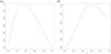Figure 10 Estimation of the difference between the conditional probabilities, between 2015 and 2013 with $\widehat{\delta }={\widehat{\delta }}_B.$ (a) $\mathrm{Prob}{ }_{2015}(U_1\le u|U_2\le u,U_3\le u)- \mathrm{Prob}{ }_{2013}(U_1\le u|U_2\le u,U_3\le u), u\in \left[\mathrm{0,1}\right]$ (see Eq. (16)). (b) $\mathrm{Prob}{ }_{2015}(U_1>u|U_2>u,U_3>u)- \mathrm{Prob}{ }_{2013}(U_1>u|U_2>u,U_3>u), u\in \left[\mathrm{0,1}\right]$ (see Eq. (17)).

5 Conclusion

In this paper, we explore the analytical skills that copula functions have to estimate conditional probabilities, especially in the tails. By adopting a family such as Joe’s copula (see [2]), it is allowed to embrace a wide range of positive dependencies, incorporated by the δ parameter ranging from δ = 1 (independence) to δ → ∞ (perfect positive dependence). In this paper we address a real problem, in which we want to quantify the ability to predict academic performance in university subjects, based on the performance in subjects/topics of the university entrance exam. We deal with annual data (around 60 observations per year) provided by the University of Campinas (2013, 2014 and 2015). We expect there to be a considerable dependence between the subjects evaluated in the entrance exam and the subjects taken during the university course, mainly in the first year of the course or in the initial educational cycles. Under this assumption we focus our study on a subject of the undergraduate course of Statistics, Calculus I and two subjects of the entrance exam related to the exact sciences: (a) Mathematics (from 2013 to 2015) and (b) Natural Sciences (in 2013 and 2014) and Physics (in 2015). We construct tail conditional probabilities (conditioned on (a) and (b)), with the purpose of inspecting extreme performances (high and low grades of Calculus I). We see that the ability to predict has gradually increased from 2013 to 2015, but this has been happening in a very poor rate. We see in Figure 10 this fact in perspective, the difference between the conditional probabilities, between 2015 (the biggest curve) and 2013 (the lowest curve) is always positive, but of at most 12%. Furthermore, as we approach to u = 0 (low notes) the difference is decreasing, see Figure 10a. And in the same way, as we approach to u = 1 (high notes) this difference is decreasing, but to a lesser degree than in the previous case, see Figure 10b. This means that for low performances there has been a less pronounced improvement than for high performances. This findings could be the result of (a) an entrance exam eventually non tuned with the preliminary notions of Calculus I, (b) very different pedagogical schemes between pre-university studies and university studies, etc. In any of these situations, it may be necessary to carry out a large-scale study and to follow up several versions of the entrance exam, for example of years subsequent to 2015, and also to follow up the performance of these students during the course.

We see in this article how the concept of copula can collaborate for the development of stochastic techniques that allow to follow year after year data bases like the one treated in this occasion. With its implementation, management mechanisms of simple implementation could be developed no requiring large sample sizes, which makes them very dynamic.

Acknowledgments

N. Romano gratefully acknowledge the financial support provided by CAPES with a fellowship of the Master Graduate Program in Statistics – University of Campinas. The authors wish to thank the three referees for their many helpful comments and suggestions on an earlier draft of this paper.

References

All Tables

All Figures

	Figure 1 (a) Percentage of population less than 15 years old (pop15) vs. percentage of the population over 75 years old (pop75). (b) Percentage of population less than 15 years old (pop15) vs. per-capita disposable income (dpi). Observations of n = 50 countries (see [6]).
In the text

	Figure 2 (a) Percentage of the population over 75 years old (pop75) vs. per-capita disposable income (dpi). (b) Scatterplot between pop15, pop75 and dpi, from red to black color in increasing order in relation to the “pop75” axis. Observations of n = 50 countries (see [6]).
In the text

Figure 3 (a) Scatterplot between ranks of pop15, ranks of pop 75 and ranks of dpi, from red to black color in increasing order in relation to the “ranks of pop75” axis. (b) Scatterplot between ranks of pop15, – ranks of pop 75 and – ranks of dpi, since ${\rho }_3^{\max }(\mathrm{pop}15,\mathrm{pop}75,\mathrm{dpi})={\rho }_3^{+}(\mathrm{pop}15,-\mathrm{pop}75,-\mathrm{dpi}).$ From red to black color in increasing order in relation to the “– ranks of pop75” axis.

In the text

	Figure 4 Data of 2013. (a) Scatterplot between Calculus I, Mathematics and Natural Sciences, from red to black color in increasing order in relation to the “Mathematics” axis. (b) Scatterplot between ranks of Calculus I, ranks of Mathematics and ranks of Natural Sciences, from red to black color in increasing order in relation to the “Ranks of Mathematics” axis.
In the text

	Figure 5 Data of 2014. (a) Scatterplot between Calculus I, Mathematics and Natural Sciences, from red to black color in increasing order in relation to the “Mathematics” axis. (b) Scatterplot between ranks of Calculus I, ranks of Mathematics and ranks of Natural Sciences, from red to black color in increasing order in relation to the “Ranks of Mathematics” axis.
In the text

	Figure 6 Data of 2015. (a) Scatterplot between Calculus I, Mathematics and Physics, from red to black color in increasing order in relation to the “Mathematics” axis. (b) Scatterplot between ranks of Calculus I, ranks of Mathematics and ranks of Physics, from red to black color in increasing order in relation to the “Ranks of Mathematics” axis.
In the text

	Figure 7 (a) $\mathrm{Prob} (U_1\le u|U_2\le u,U_3\le u)$ from equations (3) to (4), with δ = 1, 2, 4, 10, 20. (b) $\mathrm{Prob} (U_1>u|U_2>u,U_3>u)$ from equations (3) to (7), with δ = 1, 1.5, 2, 2.5, 3.
In the text

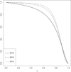	Figure 8 $\mathrm{Prob} (U_1>u|U_2\in \left[\mathrm{0.8,0.9}\right],U_3\in \left[\mathrm{0.8,0.9}\right]), u\in [\mathrm{0,1}]$ with $\widehat{\delta }={\widehat{\delta }}_B$ (see Eq. (15)).
In the text

	Figure 9 (a) $\mathrm{Prob} (U_1\le u|U_2\le u,U_3\le u), u\in [\mathrm{0,1}]$ with $\widehat{\delta }={\widehat{\delta }}_B$ (see Eq. (16)). (b) $\mathrm{Prob} (U_1>u|U_2>u,U_3>u), u\in [\mathrm{0,1}]$ with $\widehat{\delta }={\widehat{\delta }}_B$ (see Eq. (17)).
In the text

Figure 10 Estimation of the difference between the conditional probabilities, between 2015 and 2013 with $\widehat{\delta }={\widehat{\delta }}_B.$ (a) $\mathrm{Prob}{ }_{2015}(U_1\le u|U_2\le u,U_3\le u)- \mathrm{Prob}{ }_{2013}(U_1\le u|U_2\le u,U_3\le u), u\in \left[\mathrm{0,1}\right]$ (see Eq. (16)). (b) $\mathrm{Prob}{ }_{2015}(U_1>u|U_2>u,U_3>u)- \mathrm{Prob}{ }_{2013}(U_1>u|U_2>u,U_3>u), u\in \left[\mathrm{0,1}\right]$ (see Eq. (17)).

In the text

References

- Sklar A (1959), Fonctions de répartition à n dimensions et leurs marges. Publ Inst Statist Univ Paris 8, 229–231. [Google Scholar]
- Joe H (1993), Parametric families of multivariate distributions with given margins. J Multivar Anal 46, 2, 262–282. [CrossRef] [Google Scholar]
- Nelsen RB (2007), An introduction to copulas, Springer Science & Business Media, Berlin, Germany. [Google Scholar]
- Nelsen RB, Úbeda-Flores M (2012), Directional dependence in multivariate distributions. Ann Inst Stat Math 64, 3, 677–685. [CrossRef] [Google Scholar]
- García Jesús E, González-López VA, Nelsen RB (2013), A new index to measure positive dependence in trivariate distributions. J Multivar Anal 115, 481–495. [CrossRef] [Google Scholar]
- Belsley DA, Kuh E, Welsch RE (1980), Regression diagnostics, Wiley, New York, NY. [CrossRef] [Google Scholar]
- Ripley BD (2009), Stochastic simulation, Vol. 316, John Wiley & Sons, New York, NY. [Google Scholar]
- Kim G, Silvapulle MJ, Silvapulle P (2007), Comparison of semiparametric and parametric methods for estimating copulas. Comput Stat Data Anal 51, 6, 2836–2850. [CrossRef] [Google Scholar]
Cite this article as: González-López V.A, Piovesana M.C & Romano N 2019. Tail conditional probabilities to predict academic performance. 4open, 2, 18.
All Tables
Estimators of the coefficients. (i) percentage of population less than 15 years old (code 1), (ii) percentage of the population over 75 years old (code 2) and (iii) per-capita disposable income (code 3).
Direction of maximal dependence: (i) percentage of population less than 15 years old (code 1), (ii) percentage of the population over 75 years old (code 2) and (iii) per-capita disposable income (code 3).
Estimation of coefficients. On the left the bivariate Spearman’s rho coefficients (in bold letter the largest), on the right the trivariate correlations (in bold letter the largest), α m shows the direction of maximal dependence. Calculus I (subscript 1), Mathematics (subscript 2) and Natural Sciences or Physics (subscript 3).