| Issue |
4open
Volume 2, 2019
Mathematical Models
|
|
|---|---|---|
| Article Number | 15 | |
| Number of page(s) | 10 | |
| Section | Mathematics - Applied Mathematics | |
| DOI | https://doi.org/10.1051/fopen/2019008 | |
| Published online | 16 May 2019 | |
Research Article
Minimum total distance clustering and balanced distance clustering in northern Thailand's corn crop residue management system
1
Centre of Excellence in Mathematics, CHE, Bangkok
10400, Thailand
2
Center of Excellence in Mathematics and Applied Mathematics, Department of Mathematics, Faculty of Science, Chiang Mai University, Chiang Mai
50200, Thailand
* Corresponding author: This email address is being protected from spambots. You need JavaScript enabled to view it.
Received:
25
December
2018
Accepted:
19
March
2019
Abstract
The authors study the corn crop residue management system for 16 provinces in northern Thailand encompassing 127 agricultural cooperatives (co-ops), 974 corn fields and 274 customers. To solve the system's problems, we find clusters where co-ops will pick up crop residues from corn fields, process them into biomass fuel and sell the fuel to customers. Each cluster consists of a co-op, a set of corn fields and a set of customers, the latter two being on separate routes from the co-op. To minimize the system's transportation cost and balance transportation cost between clusters, we propose a mathematical model with two objective functions, construct two heuristics, and apply the two heuristics to solve the problem.
Key words: Agricultural residue management system / Northern Thailand / Heuristic / Multiple depot vehicle routing problem
© S. Phonin & C. Likasiri, Published by EDP Sciences, 2019
 This is an Open Access article distributed under the terms of the Creative Commons Attribution License (http://creativecommons.org/licenses/by/4.0/), which permits unrestricted use, distribution, and reproduction in any medium, provided the original work is properly cited.
Introduction
Thailand is one of the world's leading producers and exporters of agricultural products [1]. Major export crops include rice, sugarcane, tobacco, rubber, corn and palm oil. Cash crop cultivation areas are distributed around the country. In the north, corn is the major crop because it requires less water than other crops and is suitable for the region's mountainous terrains. Harvested corn is milled on the fields using hired milling machines, and then sold to agricultural cooperatives. By value, corn exports amounted to 13% of the country's total corn production in 2016 [2]. Yielding a total of 2.8 million metric tons, corn growing areas in northern Thailand account for 68% of the country's corn cultivation area [3]. The typical Thai corn farmer mills his corn right after harvest, leaving corn stalks, leaves, cobs and husks out in the open for later disposal.
Farm waste disposal methods include open burning, bio-composting, and biomass pellet production. The most common disposal method among northern corn farmers is open burning in the field, which produces large amounts of air pollutants. In fact, this method of elimination is believed to be a major cause of widespread air pollution problems that are endangering the health of the region's inhabitants. Thailand State of Pollution Report 2017 [4] indicated that the level of atmospheric particulate matter less than 2.5 micron in diameter (PM2.5) was in the range 115–181 μg/m3 which is higher than the national standard of 50 μg/m3 set by the Ministry of Natural Resources and Environment's Pollution Control Department. Also, particulate matter less than 10 micron in diameter (PM10) in northern provinces exceeded the national standard of 150 μg/m3, with Chiang Rai province having the highest amount of PM10 at 320 μg/m3. The region's residents suffer directly from the resultant air pollution especially particulate matter (PM10 as well as PM2.5). In 2017, the highest recorded level of PM10 in the area reached 178 μg/m3 and on 18 days in the dry season the levels of PM10 exceeded the standard value of 120 μg/m3 [5]. The highest recorded level of PM2.5 in the area that year was 116 μg/m3 and on a total of 30 days, recorded PM2.5 levels exceeded the standard value of 50 μg/m3 [6]. More recently, in April 2018, the Regional Environment Office 1 (Chiang Mai) [7] reported that PM10 level in Lampang province reached 155 μg/m3. Air pollution problems worsen every summer (March–May) due to the fact that agricultural wastes are burned on the fields without any attempt at emission control. Unless strict measures are put in place against open burning of residues, farmers are generally unwilling to use other means. Ideally, some of the waste-elimination and environmental costs should be transferred to growers. Having a power plant to cleanly burn agricultural residues will improve air quality, as this will do away with the numerous incomplete combustion burners currently used to dispose of the wastes. To reduce CO2 emissions and the air pollution affecting the lives of northerners, the government annually carries out a campaign called “No Burning for 51 Days” during March and April, and has tried different policies to curb the practice of agricultural waste burning. One of these policies, to support the transformation of waste into fuel pellets, is directly related to our case study, the corn residue transportation system in northern Thailand.
The authors study corn-crop residue management in northern Thailand with the aim to help curb the practice of in-field open burning. At present, efforts are being made to encourage the conversion of corn cobs and husks, which make up 6% and 20% of corn harvest, respectively [8], into biomass pellets with the potential to be used as bioenergy feedstock. There are works aimed at reducing biomass open burning by penalizing emissions as well as paying an incentive for biomass conversion to other energy resources [9].
In any crop residue management system, the most important cost is transportation, since the crop residues themselves cost virtually nothing. Northern Thailand's corn crop residue management system consists of farmers [or fields where corn harvest takes place and from where crop residues are sent (or picked up by the co-op) for processing]; co-ops, which process the harvested crop, turn corn cobs and husks into biomass pallets and offer both corn kernels and biomass pellets for sale; and customers, who agree to purchase the biomass fuel from the co-ops.
In this study, an optimization model is constructed to find clusters/routings comprising a co-op (depot), and two types of clients, namely: (1) farmers (or pickup customer), and (2) factories (or delivery customers). In our problem, pickup customers are served, the vehicle comes back fully loaded to the depot and then leaves again with the processed products to be dropped off at delivery customers. There are multiple agricultural cooperatives in the system. We are interested in finding the routing via Multiple Depot Vehicle Routing Problem with Backhaul (MDVRPB) with two alternative objective functions: to minimize the total distance in all routes, and to balance the total distance in each route so that each depot will bear equal share of the transportation cost. The later objective plays a very important role in policy setting. Since the total transportation cost in this objective is generally higher than the cost obtained from the first objective, the difference can be used to determine an appropriate incentive for corn residue conversion to biomass energy resources. Here, routes are identified under the following restrictions: each route begins and ends at the same depot; each customer belongs to only one route; each route comprises two types of clients i.e., the farmers and the factories, and the co-ops serving as depots in the case study; and the total demand of the assigned customer cannot exceed the depot's capacity. In the approach of the proposed heuristics, we have investigated both split and no split deliveries but found not positive results on the split deliveries. Hence, in this work, split deliveries are not allowed, but they will be investigated further in future work.
Literature review
The Vehicle Routing Problem (VRP), a well-known combinatorial optimization problem, is concerned with designing routes to serve a set of customers subject to vehicle and customer restrictions. VRP was first introduced by Dantzig and Ramser [10], who proposed a mathematical formulation and algorithm for finding the optimal routing for a fleet of gasoline delivery trucks between a bulk terminal and the service stations supplied by the terminal. Eksioglu et al. [11] classified the literature of VRP by five different aspects consisting of: (1) type of study, (2) scenario characteristics, (3) problem physical characteristics, (4) information characteristics, and (5) data characteristics. Among the first researchers to study a variety of VRP, Solomon [12] studied the VRP with Time Windows (VRPTW) constraints, which are the constraints that considerably complicate the problem. Because of this, the topic was subsequently extensively studied. Sexton and Bodin [13] were the first to examine the pickup and delivery problem with constraint on delivery times. They proposed heuristics to find and improve the initial route. Savelsbergh and Sol [14] gave an extensive survey on the problem types and solution methods of pickup and delivery problems, which involve transportation of loads from origin to destination without transshipment node. In their survey, VRP is considered static whereas pickup and delivery problems are often dynamic. Hence, in pickup and delivery problems, the concept of depots vanished. However, Parragh et al. [15, 16] later conducted another survey on pickup and delivery problems. In their survey, there are no dynamic concepts in pickup and delivery problem. The problems can be classified into two groups, VRP with Backhaul (VRPB), where the transportation is done from and to the depot, and VRP with Pickup and Delivery (VRPPD), where the loads are transported between pickup and delivery locations. For a recent literature review on VRPB, we refer the interested reader to work of Koç and Laporte [17].
Toth and Vigo [18] offered an exact algorithm for VRPB where pickup customers are visited after all delivery customers have been visited. The lower bounds obtained consist of Lagrangian and dropping capacity constraint lower bounds. Salhi and Nagy [19] investigated both single VRPB and multiple VRPB. In their work, pickups and deliveries can be done in mixed order. Their proposed method is done by solving VRP for delivery customers and inserting pickup customers to the route. In Tavakkoli-Moghaddam et al. [20], pickup customers also needed to be served first and the authors used local search and GA to solve this NP-hard problem. In Nagy et al.'s [21] study of VRP with divisible deliveries and pickups, even though a customer might have both pickup and delivery demand, the demands are served on two separate visits. They also studied the savings from satisfying pickups and deliveries separately instead of simultaneously.
Another extension of VRP is called Multiple Depot Vehicle Routing Problem (MDVRP). Currently, fewer studies have been published on MDVRP than on classic VRP. Baldacci and Mingozzi [22] proposed an exact method for solving an extended model of Capacitated VRP (CVRP) including Heterogeneous VRP (HVRP), Site-Dependent VRP (SDVRP), and MDVRP. Bounding procedures offered in this work are based on the LP-relaxation and Lagrangian relaxation. Contardo and Martinelli [23] also proposed an exact algorithm for solving Capacitated MDVRP (CMDVRP) under length-of-route constraints. Their algorithm involved column-and-cut generation and a new set of valid inequalities. Consequently, compared to the existing methods, it produced tighter lower bounds for unsolved problems and solved some hard instances optimally.
Only in small instances can exact algorithm solve general MDVRP within reasonable execution time. Metaheuristic methods have been proposed to solve large-size versions of the problem. These methods are capable of finding near-optimal solutions within reasonable time, but they cannot guarantee an optimal solution. To construct the heuristics, we study related works on solving MDVRP using metaheuristics. Lim and Wang [24] proposed algorithms for solving MDVRP with exactly one vehicle in each depot. This scenario is a useful variant of MDVRP since it can be extended to any number of available vehicles. They offered both 1- and 2-stage approaches. Whereas their 1-stage approach conducts the assignment and routing procedures simultaneously, the 2-stage approach solves the assignment problem and then applies TSP to find the routing schedule independently. Their algorithms are partitioned into assignment method and routing method. Crevier et al. [25] studied MDVRP with Inner-Depot route (MDVRPI) where routing can start and end at a different depot. Routings in the proposed algorithm are generated based on tabu search algorithm. A set of benchmark instances for this problem is also introduced in this work. Kuo and Wang [26] proposed a variable neighborhood search for solving MDVRP with Loading Cost (MDVRPLC). Their heuristics combined stochastic method for the initial solution, neighborhood search and simulated annealing to improve the solution. Allahyari et al. [27] proposed a MDVRP where only some customers need to be visited. The demand of those who are not visited are satisfied by the customer in the tour. The metaheuristics are constructed based on greedy randomized adaptive search, iterated local search and simulated annealing. Oliveira et al. [28] decomposed the problem into subproblems with a single depot, simultaneously obtained the partial solutions and formed a complete solution to the problem via the proposed method similarly to that of GA and local search. Wang et al. [29] solved split delivery MDVRP with minimum service time requirement. Their objective is to minimize the duration of the longest route. After an initial feasible solution is constructed without splits, the improved solution is found by splitting service time to reduce the longest route, and to satisfy the minimum service time requirement.
Corn crop residue data collection
Locations of corn fields, co-ops and customers are mapped out and then the shortest distances between any two locations are identified using Google Map. The corn crop residue management system for 16 provinces in northern Thailand covers 974 fields, 127 co-ops, and 274 customers, for a total of 1375 locations. Northern Thailand is located between 17° 10′–20° 27′ North latitude and 97° 22′–100° 00′ East longitude.
Optimization model
In order to construct the optimization model, we first define some parameters and decision variables, then we state the two objective functions followed by constraints.
Parameters and decision variables
The model's parameters are denoted as follows: r is the number of co-ops/clusters; m is the number of corn fields; n is the number of customers; K is a set of co-ops/clusters, K = {1, …, r}; P is a set of corn fields, P = {r + 1, …, r + m};  is a set of customers, D = {r + m + 1, …, r + m + n}; V is the set of all locations
  ; c
ij
is the distance between ith and jth vertices; f
k
is the fixed cost of opening the kth co-op; s
i
is the supply at ith corn field; d
i
is the demand at ith customer; and q
k
is the capacity of kth co-op. The decision variables are:
; c
ij
is the distance between ith and jth vertices; f
k
is the fixed cost of opening the kth co-op; s
i
is the supply at ith corn field; d
i
is the demand at ith customer; and q
k
is the capacity of kth co-op. The decision variables are:
-

-
-
 is the load of the kth vehicle (i.e., the capacity of the kth co-op) when departing from ith vertex.
Objective function
The two main optimization objectives in this work are to minimize the traveled distance in the system and minimize traveled distance differences among clusters.
The first objective, to minimize the total distance traveled, can be written as (1)The second objective, to balance the cost between clusters, can be written as
 (2)
(2)
Constraints
Each cluster needs to have a single co-op that serves the entire sets of corn fields and customers. A co-op makes the rounds of all the corn fields in a single routing and serves all the customers in another single routing. We therefore do not consider the capacities of the trucks used for pickups and deliveries. The constraints of this problem can be described as follows:
-
The vehicle at each co-op can be used when that co-op is open:
 (3)
(3)
 (4)
(4) -
Each route from corn field or customer ends at the co-op serving as the start of that route:
 (5)
(5)
 (6)
(6) -
The kth route only starts from the kth co-op:
 (7)
(7) -
Each corn field or customer can only be in one cluster:
 (8)
(8) -
The flow conservation of each vertex, i.e., the number of entering arcs of each vertex, is equal to the number of that vertex's leaving arcs:
 (9)
(9) -
Since corn residues need to be processed at the depots before delivery to customers can be made, the corn fields cannot be directly connected to the customers in each route:
 (10)
(10) -
The combined supply from corn fields on each route cannot exceed the capacity of the co-op serving that route and the combined demand from customers cannot exceed the total amount of corn residues available on that route:
 (11)
(11)
 (12)
(12) -
The subtour elimination constraints:
 (13)
(13)
 (14)
(14)
 (15)
(15)
 (16)
(16)


Heuristics construction
The problem of clustering corn fields, customers and co-ops comprising 1375 vertices cannot be solved via CPLEX. In order to find a best solution, we work to improve existing greedy algorithm-based heuristics. In both proposed heuristics, the corn fields must be clustered first in order to determine the total available supplies before the customers are visited. In the first heuristics, called the Minimum Distance and Supply Ratio (MDSR), a corn field (or customer) will be assigned to a co-op/cluster if the ratio between its distance to the cluster and the size of its supply is the lowest and its supply does not exceed the remaining capacity of the cluster's co-op. The process of this heuristic is illustrated in Figure 1. In the second heuristic, called the Minimum Distance and Supply Ratio with Balancing co-op (MDSRB), the co-op serves the supplier that has the lowest ratio between distance to the cluster and size of supply, provided that the size of this supplier's supply does not exceed the co-op's remaining capacity. This heuristic also aims to evenly spread the closest supplier of each co-op. Consequently, the co-ops are sequentially assigned to the as-yet unassigned corn fields. The process of the second heuristic is illustrated in Figure 2.
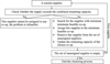 |
Figure 1 The process of MDSR heuristic. |
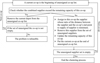 |
Figure 2 The process of MDSRB heuristic. |
Minimum Distance and Supply Ratio (MDSR)
The assignment strategy of this heuristic is to assign a supplier (customer) to the cluster only if the ratio between its minimum distance to the cluster and its supply (demand) is the smallest. Call the co-op of this cluster the minimum feasible co-op. Hence, for each supplier i in this algorithm, we assign the supplier to its minimum feasible co-op. For each remaining suppliers, repeat this process until all suppliers have been assigned to co-ops. The proposed algorithm can be written as follows;
	While the unassigned supplier set is not empty,
	 Find the supplier located nearest to its minimum feasible co-op
	 If the size of this supplier's supply exceeds the remaining capacity of every co-op,
	    this supplier cannot be assigned to any co-op, the problem is infeasible.
	 Else,
	   assign this supplier to the cluster with its minimum feasible co-op,
	   remove the supplier from the unassigned supplier set, and
	   update the remaining capacity of the chosen co-op.
	 End.
	 Repeat this process until the unassigned supplier set is empty.
	End
Minimum Distance and Supply Ratio with Balancing co-op (MDSRB)
This heuristic's assignment strategy is to assign the cluster to a supplier (customer) with the lowest ratio between minimum distance to the cluster and size of supply (demand). This supplier is called the minimum feasible supplier of this cluster. In other words, in this algorithm, we assign to each cluster its minimum feasible supplier. We assign a supplier to an unassigned co-op until the unassigned co-op list is empty, and repeat this process until all suppliers have been assigned to co-ops. The proposed algorithm can be written as follows;
	Do while the unassigned supplier set is not empty,
	 While the list of unassigned co-ops is not empty
	  If the size of each supplier's supply exceeds the remaining capacity of co-op j,
	   remove co-op j from the unassigned co-op list.
	   If the unassigned co-op list is not empty,
	     move to the next co-op on the list.
	   Else,
	     the problem is infeasible.
	   End.
	 Else,
	   assign co-op j to its minimum feasible supplier,
	   remove the supplier from the unassigned supplier set,
	   update the remaining capacity of co-op j,
	   and move co-op j to the end of the unassigned co-op list.
	  End.
	  Move to the next co-op in the list.
	 End.
	Move to the next unassigned supplier.
	End.
Computational results via the proposed heuristics
To test the models, we formulate a model with two objective functions on AIMMS where the model is optimally solved via CPLEX. The optimal route and its associated total transportation cost are found in small instances with execution time of no more than 24 h. The sizes of the test problems are 6 × 3 × 3 (6 suppliers × 3 co-ops × 3 customers), 6 × 3 × 4, 6 × 3 × 5 and 6 × 3 × 6. The solutions to these problems are compared with the solution obtained from the two proposed heuristics. All sets of problems are simulated and solved on Intel® Xeon® CPU 2.30 GHz 2.29 GHz (two processors) with 64 GB of RAM. In each case, 30 problems are generated using normal distribution since we observe that the real-world data are normal. The distances between two nodes are normally generated with the mean at  and Standard Deviation (SD) of
  . The capacities of the co-ops are generated from normal distribution with the mean at 1000 and SD of 200, combined supply from all suppliers at 60% of combined capacities of all co-ops while the combined demand of the customers is 60% of the combined supply from all suppliers. The supplies from suppliers are normally generated with the mean at 180 and SD of 54 while the demands of customers are normally generated with different mean depending on the number of suppliers and with SD being 30% of mean. All problems’ fixed cost is set to be zero.
In Table 1, the average total distance in each cluster found from the optimal solution with two objective functions, MDSR and MDSRB are shown along with average processing times. MDSR is constructed to solve the first objective function, MDSRB to solve the second objective function. As expected, the total distance traveled in the system found via the model with the first objective function is shorter than that obtained from both heuristics in all problem sizes. We compare the SD of each solution to find the best balanced distance in each cluster. The balanced distance clusters obtained from the model with the second objective function yields the worst total distance. It can be concluded from the large gaps in the SD shown in the table that the second objective function results in clusters with a lot more balanced distance traveled. For problems with 3, 4, 5 and 6 customers, the number of cases having only 2 out of 3 co-ops opened are 25, 20, 22 and 26 cases out of 30 cases, respectively, in the first objective optimal solutions. That number is much smaller at 5, 9, 6 and 9, respectively, if we solve with MDSR heuristic. However, when we solve the problem with the second objective, all co-ops are opened regardless of the method used.
Computational results for problem size six suppliers, three co-ops, and c customers.
To compare the heuristics in larger instances that cannot be solved optimally using the two models, 30 problems in sizes 3000 × 100 × 100, 3000 × 100 × 200, 3000 × 100 × 300, 3000 × 100 × 400 and 3000 × 100 × 500 are normally generated and solved on Intel® Xeon® CPU E5-2667 v4 @ 3.20 GHz 3.20 GHz (two processors) with 64 GB of RAM., where the distances between suppliers, customers and co-ops are generated in the interval [1300]. The suppliers’ supplies and customers’ demands are in the range of [0, 3500] and [3000, 12 000], respectively. The capacities of the co-ops fall in the [15 000, 50 000] interval. All problems’ fixed cost is set to be zero. Data generated are provided via http://dx.doi.org/10.17632/gww7sf5m6m. Results are shown in Table 2. Note that all co-ops are opened in all these cases.
Computational results for problem size 3000 suppliers, 100 co-ops, and c customers.
Solving crop residue transportation via the proposed heuristics
We solve a real-world problem using MDSR and MDSRB heuristics. The results are shown in Table 3. The total traveled distance obtained from MDSR is shorter than that obtained from MDSRB because MDSR searches all corn fields (or customers) for the co-ops with the lowest distance-to-the-cluster-to-supply-size ratio with the nearest corn fields being assigned to co-ops. The second and third columns show the maximum and minimum traveled distances of all the clusters, respectively. The fourth column shows the average traveled distance in each cluster while the fifth column shows the standard deviation of all the clusters’ traveled distances. We observe that the minimum traveled distance from MDSR is 0, i.e., some co-ops are not opened in the MDSR solution, whereas every co-op is opened in the MDSRB solution. The number of opened co-op is also given in Table 3. The reason is that MDSRB attempts to balance total traveled distance in each cluster and therefore all co-ops have to be opened.
Corn crop residue transportation results for 16 northern Thailand provinces.
Conclusions and discussions
This work proposes mathematical formulations for assigning two different types of clients to routings via capacitated multi-depot vehicle routing problem. One of the objectives is to find the transportation system with minimum total distance traveled, where each route in the system contains only one depot whose capacity is sufficient for the supplies/demands in that cluster. We propose two objective functions for the problem with the same set of constraints, that each route has one depot dealing with all the supplies/demands. The first model is called CMVRP2C where the total cost is minimized. The second model is called CMVRPB where the balance of the transportation costs of each route is the main objective. The optimal solutions of CMVRP2C and CMVRPB can be obtained only in small-size problems.
Two heuristics, MDSR and MDSRB, are constructed to find the corn crop residue management clusters which are larger problem. The heuristics’ assignment strategy is to first pair each cluster's co-op with a corn field (or customer) with the lowest ratio between its minimum distance to the cluster and the size of its supply (demand). If there are two locations with the same supply size, the nearest location will be assigned first. With MDSR heuristic, all corn fields or customers are to be found and assigned to the nearest co-op, thus the co-ops located close to corn fields or customers are chosen but co-ops located far away from them are not. With both heuristics, all corn fields will be clustered first. The total supplies gathered at the co-op will be equal to the capacity of that co-op. Customers are then clustered to the co-op to make sure that all the customer demand in the cluster will be met. If there is excess supply, it will be left at the co-op. Two interesting topics are currently being investigated by the authors: when the capacity of the trucks serving the system is considered, and when the clusters of corn fields and customers are built simultaneously.
Acknowledgments
This research is supported by the Center of Excellence in Mathematics and Applied Mathematics, Department of Mathematics, Faculty of Science, Chiang Mai University. Appreciation is extended to the Centre of Excellence in Mathematics, CHE for financial support. Corn production data are provided courtesy of Thailand's Energy Technology for Research Center.
References
- WTO (World Trade Organization), World Trade Statistical Review 2017. https://www.wto.org/english/res_e/statis_e/wts2017_e/wts2017_e.pdf (Accessed on 10 April 2019). [Google Scholar]
- Office of Agricultural Economics, Major Agricultural Commodities Overview and Outlook 2018 (สถานการณ์สินค้าเกษตรที่สำคัญและแนวโน้มปี 2561) http://oldweb.oae.go.th/download/document_tendency/agri_situation2561.pdf (Accessed on 10 April 2019) (in Thai). [Google Scholar]
- Office of Agricultural Economics, Agricultural statistics of Thailand 2016 (สถิติการเกษตรของประเทศไทยปี 2559). http://oldweb.oae.go.th/download/download_journal/2560/yearbook59.pdf. (Accessed on 10 April 2019) (in Thai). [Google Scholar]
- The Pollution Control Department of Thailand, Current situation and management of air and noise pollutions in Thailand 2016 (สถานการณ์และการจัดการปัญหามลพิษทางอากาศและเสียงของประเทศไทย ปี 2559). http://www.oic.go.th/FILEWEB/CABINFOCENTER3/DRAWER056/GENERAL/DATA0001/00001018.PDF (Accessed on 10 April 2019) (in Thai). [Google Scholar]
- Regional Environment Office 1 (Chiang Mai), Smog situation report 2017, (รายงานสถานการณ์หมอกควัน ปี 2560). http://www.reo01.mnre.go.th/th/information/list/254 (Accessed on 10 April 2019). (in Thai). [Google Scholar]
- Greenpeace Thailand, PM2.5 pollutions in Thailand’s urban areas: January–June 2017 (มลพิษฝุ่นละอองขนาดเล็กไม่เกิน 2.5 ไมครอน (PM2.5) ของเมืองในประเทศไทย ช่วงเดือนมกราคม-มิถุนายน พ.ศ.2560), https://www.greenpeace.or.th/s/right-to-clean-air/PM2.5-in-Thailand_Jan-Jun2017.pdf. (Accessed on 10 April 2019) (in Thai). [Google Scholar]
- Regional Environment Office 1 (Chiang Mai), Announcement: Air Situation Exceeds Standard Values, (ประกาศสถานการณ์อากาศเกินค่ามาตรฐาน). http://www.reo01.mnre.go.th/th/news/detail/12426/ (Accessed on 9 April 2019) (in Thai). [Google Scholar]
- Sasujit K, Sanpinit W, Wongrin N, Dussadee N (2015), A study of the process of densification of corn cob and corn husk briquettes by cold extrusion technique using starch with lime mixed as binder. Thaksin Univ J 18, 1, 1–14. (in Thai). [Google Scholar]
- Ghani NAMAA, Vogiatzis C, Szmerekovsky J (2018), Biomass feedstock supply chain network design with biomass conversion incentives. Energy Policy 116, 39–49. https://doi.org/10.1016/j.enpol.2018.01.042. [Google Scholar]
- Dantzig GB, Ramser JH (1959), The truck dispatching problem. Manag Sci 6, 1, 80–91. https:doi.org/10.1287/mnsc.6.1.80. [Google Scholar]
- Eksioglu B, Vural AV, Reisman A (2009), The vehicle routing problem: A taxonomic review. Comput Ind Eng 57, 4, 1472–1483. https://doi.org/10.1016/j.cie.2009.05.009. [Google Scholar]
- Solomon MM (1984), Algorithms for the vehicle routing and scheduling with time window constraints. Oper Res 35, 2, 254–265. https://doi.org/10.1287/opre.35.2.254. [Google Scholar]
- Sexton TR, Bodin LD (1985), Optimizing single vehicle many-to-many operations with desired delivery times: II. Routing Transp Sci 19, 4, 411–435. https://doi.org/10.1287/trsc.19.4.411. [CrossRef] [Google Scholar]
- Savelsbergh MWP, Sol M (1995), The general pickup and delivery problem. Transp Sci 29, 1, 17–29. https://doi.org/10.1287/trsc.29.1.17. [Google Scholar]
- Parragh SN, Doerner KF, Hartl RF (2008), A survey on pickup and delivery problems Part I: Transportation between customers and depot. J Betriebswirtsch 58, 1, 21–51. https://doi.org/10.1007/s11301-008-0033-7. [CrossRef] [Google Scholar]
- Parragh SN, Doerner KF, Hartl RF (2008), A survey on pickup and delivery problems Part II: Transportation between pickup and delivery locations. J Betriebswirtsch 58, 1, 81–117. https://doi.org/10.1007/s11301-008-0036-4. [CrossRef] [Google Scholar]
- Koç Ç, Laporte G (2018), Vehicle routing with backhauls: Review and research perspectives. Comput Oper Res 91, 79–91. https://doi.org/10.1016/j.cor.2017.11.003. [Google Scholar]
- Toth P, Vigo D (1997), An exact algorithm for the vehicle routing problem with backhauls. Transp Sci 31, 4, 372–385. https://doi.org/10.1287/trsc.31.4.372. [CrossRef] [Google Scholar]
- Salhi S, Nagy G (1999), A cluster insertion heuristic for single and multiple depot vehicle routing problems with backhauling. J Oper Res Soc 50, 10, 1034–1042. https://doi.org/10.1057/palgrave.jors.2600808. [Google Scholar]
- Tavakkoli-Moghaddam R, Saremi AR, Ziaee MS (2006), A memetic algorithm for a vehicle routing problem with backhauls. Appl Math Comput 181, 1049–1060. https://doi.org/10.1016/j.amc.2006.01.059. [Google Scholar]
- Nagy G, Wassan NA, Speranza MG, Archetti C (2015), The vehicle routing problem with divisible deliveries and pickups. Transp Sci 49, 2, 271–294. https://doi.org/10.1287/trsc.2013.0501. [CrossRef] [Google Scholar]
- Baldacci R, Mingozzi A (2009), A unified exact method for solving different classes of vehicle routing problems. Math Program 120, 347–380. https://doi.org/10.1007/s10107-008-0218-9. [Google Scholar]
- Contardo C, Martinelli R (2014), A new exact algorithm for the multi-depot vehicle routing problem under capacity and route length constraints. Discrete Optim 12, 129–146. https://doi.org/10.1016/j.disopt.2014.03.001. [CrossRef] [Google Scholar]
- Lim A, Wang F (2005), Multi-depot vehicle routing problem: A one-stage approach. IEEE Trans Autom Sci Eng 2, 4, 397–402. https://doi.org/10.1109/TASE.2005.853472. [Google Scholar]
- Crevier B, Cordeau J-F, Laporte G (2007), The multi-depot vehicle routing problem with inter-depot routes. Eur J Oper Res 176, 756–773. https://doi.org/10.1016/j.ejor.2005.08.015. [Google Scholar]
- Kuo Y, Wang C-C (2012), A variable neighborhood search for the multi-depot vehicle routing problem with loading cost. Expert Syst Appl 39, 6949–6954. https://doi.org/10.1016/j.eswa.2012.01.024. [Google Scholar]
- Allahyari S, Salari M, Vigo D (2015), A hybrid metaheuristic algorithm for the multi-depot covering tour vehicle routing problem. Eur J Oper Res 242, 756–768. https://doi.org/10.1016/j.ejor.2014.10.048. [Google Scholar]
- Oliveira FB, Enayatifar R, Sadaei HJ, Guimaraes FG, Potvin J (2016), A cooperative coevolutionary algorithm for the Multi-Depot Vehicle Routing Problem. Expert Syst Appl 43, 117–130. https://doi.org/10.1016/j.eswa.2015.08.030. [Google Scholar]
- Wang X, Golden B, Wasil E, Zhang R (2016), The min–max split delivery multi-depot vehicle routing problem with minimum service time requirement. Comput Oper Res 71, 110–126. https://doi.org/10.1016/j.cor.2016.01.008. [Google Scholar]
Cite this article as: Phonin S & Likasiri C 2019. Minimum total distance clustering and balanced distance clustering in northern Thailand’s corn crop residue management system. 4open, 2, 15.
All Tables
Computational results for problem size six suppliers, three co-ops, and c customers.
Computational results for problem size 3000 suppliers, 100 co-ops, and c customers.
All Figures
|
Figure 1 The process of MDSR heuristic. |
| In the text | |
|
Figure 2 The process of MDSRB heuristic. |
| In the text | |