| Issue |
4open
Volume 5, 2022
Logical Entropy
|
|
|---|---|---|
| Article Number | 2 | |
| Number of page(s) | 14 | |
| Section | Physics - Applied Physics | |
| DOI | https://doi.org/10.1051/fopen/2021005 | |
| Published online | 25 January 2022 | |
Research Article
Quantum logical entropy: fundamentals and general properties
1
Faculty of Interdisciplinary Studies, Bar-Ilan University, Ramat Gan 5290002, Israel
2
Faculty of Engineering and the Institute of Nanotechnology and Advanced Materials, Bar-Ilan University, Ramat Gan 5290002, Israel
3
School of Computer Science and Engineering, The Hebrew University, Jerusalem 91904, Israel
* Corresponding author: This email address is being protected from spambots. You need JavaScript enabled to view it.
Received:
3
August
2021
Accepted:
1
November
2021
Abstract
Logical entropy gives a measure, in the sense of measure theory, of the distinctions of a given partition of a set, an idea that can be naturally generalized to classical probability distributions. Here, we analyze how this fundamental concept and other related definitions can be applied to the study of quantum systems with the use of quantum logical entropy. Moreover, we prove several properties of this entropy for generic density matrices that may be relevant to various areas of quantum mechanics and quantum information. Furthermore, we extend the notion of quantum logical entropy to post-selected systems.
Key words: Logical entropy / Quantum logical entropy / Distinctions / Post-selected systems
These two authors contributed equally to this work.
© B. Tamir et al., Published by EDP Sciences, 2022
 This is an Open Access article distributed under the terms of the Creative Commons Attribution License (http://creativecommons.org/licenses/by/4.0/), which permits unrestricted use, distribution, and reproduction in any medium, provided the original work is properly cited.
1 Introduction
Entropy is one of the paramount concepts in probability theory and physics. Even though information does not seem to have a precise definition, the Shannon entropy is seen as an important measure of information about a system of interest, while the Gibbs entropy plays a similar role in statistical mechanics. A possible and, in a sense, natural extension of these classical measures to the quantum realm is the von Neumann entropy. Despite playing a fundamental role in many applications in quantum information, the von Neumann entropy was criticized on several different grounds [1–3]. In a nutshell, while classical entropy indicates one’s ignorance about the system [4], quantum entropy seems to have a fundamentally different flavor, corresponding to an a priori inaccessibility of information or the existence of non-local correlations. In this perspective, classical entropy concerns subjective/epistemic indefiniteness, while quantum entropy is associated with some form of objective/ontological indefiniteness [5], although this reasoning can be contested. To address conceptual problems like this one, the non-additive Tsallis entropy and other measures were proposed [1, 6, 7].
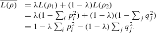
Classical logical entropy was recently introduced by Ellerman [8, 9] as an informational measure arising from the logic of partitions. As such, this entropy gives the distinction of partitions of a set U. A partition π is defined as a set of disjoint parts of a set, as exemplified in Figure 1a. The set can be thought of as being originally fully distinct, while each partition collects together blocks whose distinctions are factored out. Each block represents elements that are associated with an equivalence relation on the set. Then, the elements of a block are indistinct among themselves while different blocks are distinct from each other, given an equivalence relation.
 |
Figure 1 Pictorial representation of a set with a partition and its distinction. (a) A set U with six elements ui is divided in a partition π with three blocks (green areas). (b) The set U × U has each of its points characterized by a square in a 2D mesh. Points that belong to dit(π), i.e., pairs whose components belong to different blocks are colored in green. |
With these concepts in mind, it seems that the extension of this framework of partitions and distinctions to the study of quantum systems may bring new insights into problems of quantum state discrimination, quantum cryptography, and quantum channel capacity. In fact, in these problems, we are, in one way or another, interested in a distance measure between distinguishable states, which is exactly the kind of knowledge the logical entropy is associated with.
This work is an updated and much extended version of a previous preprint that proposed the study of quantum logical entropy [10]. In this new version, like in the original one, we focus mostly on basic definitions and properties of this quantity. Other advanced topics were either treated in previous research, like in [11], or are left for future investigation. However, as it will be further elaborated upon across the text, the results presented here lay the groundwork for various theoretical applications – even for scenarios involving post-selected systems.
To set the framework, we start with a brief overview of classical logical entropy. For that, consider a finite set U and a partition π = {Bi} of U, where each block Bi is a disjoint part of U. Moreover, denote by dit(π) the distinction of the partition π, i.e., the set of all pairs (u, u′) ∈ U × U such that u and u′ are not in the same block Bi of the partition π, as illustrated in Figure 1b.
The logical entropy Lπ (U) is defined as 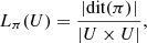 (1)where
  denotes the cardinality of the set. In other words, Lπ (U) is the probability of getting elements from two different blocks Bi after uniformly drawing two elements from U. Therefore, it is a measure of average distinction.
If each element of U is assumed to be equally probable, we can write 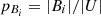 and, thus,
  (2)
(2)
Furthermore, if a probability pk is assigned to each element uk ∈ U, the above expression can be applied to the partition π = 1U with element-blocks given by {ui}. This leads to  (3)
(3)
Therefore, L({pi}) is the probability to draw two different elements ui consecutively. To generalize it even further, one may consider an arbitrary set U with a countable number of blocks. In this case, the idea of logical entropy is extended to countable probability distributions.
Starting from this definition, other concepts, like logical divergence, conditional logical entropy, and mutual logical information [8], can also be introduced along the same lines.
It should be noted that the formula for logical entropy is rooted in the history of information theory, preceding by at least a century its relation to the logic of partitions introduced by Ellerman. In fact, it can be traced back to Gini’s index of mutability [12]. Also, Polish Enigma crypto-analysts and, later, Turing used the term “repeat rate” [13–15], which is just the complement of the logical entropy. Moreover, it coincides with the Tsallis entropy of index 2 and, as a result, resembles the information measure suggested by Brukner and Zeilinger [1, 2] and Manfredi [7] for applications in quantum mechanics.
Here, we follow standard methods from quantum information (e.g., [16]) to extend the notion of logical entropy to quantum states. In this approach, the set U becomes the state of a quantum system, i.e., an element of a Hilbert space. With that, besides adding new results, we generalize the ones originally presented in [17], supporting them with formal proofs regarding quantum density matrices. We hope that the discussion we present will shed new light on this intriguing informational measure.
Since the writing of the original manuscript [10], additional works in this area have elaborated on the topic [18–23]. Still, we expect that the updates added here will provide new insights into the subject. In fact, within the next section, we present a new road to the introduction of quantum logical entropy that makes its connection with the idea of partitions present in the classical definition more evident. After that, in the section with the properties of quantum logical entropies, we prove some results that were not present in the original manuscript and simplify the proofs to others that were already on it whenever possible. Moreover, we added a section where new definitions of logical entropy for post-selected systems are introduced. To conclude this work, we further discussions some aspects of our study in the final section.
2 Quantum logical entropy
Every projection-valued measure (PVM) defines a partition π in a Hilbert space in the sense that it provides a direct-sum decomposition of the space [24, 25]. In fact, recall that a PVM is characterized by parts Bi = |bi〉〈bi| such that  . Then, the probability that two consecutive measurements of copies of a state ρ in such a Hilbert space will belong to distinct parts is
 ![Mathematical equation: $$ {L}_{\pi }(\rho )\equiv \sum_i \mathrm{tr}({B}_i\rho )[1-\mathrm{tr}({B}_i\rho )]. $$](/articles/fopen/full_html/2022/01/fopen210005/fopen210005-eq7.gif) (4)
(4)
Observing that tr(Bi
ρBi) = tr(Bi
ρ) and Bi
ρBi = tr(Bi
ρ)Bi, which implies that [tr(Bi
ρBi)]2 = tr(Bi
ρBi)2, the quantity Lπ(ρ) can be rewritten as ![Mathematical equation: $$ \begin{array}{ll}{L}_{\pi }(\rho )& =\sum_i \mathrm{tr}({B}_i\rho {B}_i)-\sum_i [\mathrm{tr}({B}_i\rho {B}_i){]}^2\\ & =\mathrm{tr}\left(\sum_i {B}_i\rho {B}_i\right)-\mathrm{tr}\left[\sum_i ({B}_i\rho {B}_i{)}^2\right]\\ & =\mathrm{tr}\rho \mathrm{\prime}-\mathrm{tr}(\rho \mathrm{\prime}{)}^2\\ & =\mathrm{tr}[\rho \mathrm{\prime}(I-\rho \mathrm{\prime})],\end{array} $$](/articles/fopen/full_html/2022/01/fopen210005/fopen210005-eq8.gif) (5)where ρ′ = ∑i(Bi
ρBi) is the measured density matrix ρ with the PVM associated with π. The operator ρ′ is sometimes referred to as Lüders mixture (see, e.g., [26]) since it was introduced by Lüders [27] as a generalization of the state update rule proposed by von Neumann in his seminal book [28].
(5)where ρ′ = ∑i(Bi
ρBi) is the measured density matrix ρ with the PVM associated with π. The operator ρ′ is sometimes referred to as Lüders mixture (see, e.g., [26]) since it was introduced by Lüders [27] as a generalization of the state update rule proposed by von Neumann in his seminal book [28].
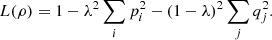
Expression (4) already defines a logical entropy for the state ρ for a given partition π (characterized by a PVM), as represented in Figure 2. Observe that this definition can be applied even in cases of coarse PVMs, i.e., PVMs with degeneracy. In this sense, and perhaps somewhat differently from the von Neumann entropy, the logical entropy has a clear operational meaning directly associated with its definition.
 |
Figure 2 Representation of the probability distribution used in the definition of quantum logical entropy. Any state ρ, together with a partition characterized by a PVM, which is associated with an orthonormal basis in the corresponding Hilbert space, defines a probability distribution. This is the case even in case of coarse (i.e., degenerate) PVMs, as illustrated by the yellow partition. These distributions allow the introduction of (PVM-dependent) logical entropies for quantum systems. |
The dependency on PVMs should not come as a surprise since, even classically, as already seen, the logical entropy, in general, depends on the partition. However, if we wish to have a PVM-independent quantum logical entropy, we can define  (6)
(6)
While this is not the only possible definition, it coincides with the one that is typically considered in the literature, as shown next. It is, also, in a certain sense, a “natural” choice. In fact, it turns out that the PVM that minimizes Lπ (ρ) is the one associated with a basis for which ρ is diagonal, in which case ρ = ρ′. To see that, let ρ = ∑ij
ρij|i〉〈j| be a representation of ρ in the basis associated with the projectors Bi. In this same basis, ρ′ = ∑i
ρii|i〉〈i|. Moreover,  (7)which implies that Lπ(ρ) = 1 − trρ
2 + ∑i ∑j≠i|ρij|2, which is minimized whenever ρ is diagonal in the basis associated with the projectors Bi. Since this is the case for every non-degenerate PVM, we conclude that
(7)which implies that Lπ(ρ) = 1 − trρ
2 + ∑i ∑j≠i|ρij|2, which is minimized whenever ρ is diagonal in the basis associated with the projectors Bi. Since this is the case for every non-degenerate PVM, we conclude that ![Mathematical equation: $$ L(\rho )=\mathrm{tr}[\rho (I-\rho )]. $$](/articles/fopen/full_html/2022/01/fopen210005/fopen210005-eq11.gif) (8)
(8)
This is the expression that was defined as the quantum logical entropy in the original version of this work [10] and has, ever since, been used in the literature (see, e.g., [23]). In this update of the work, however, we introduce the quantum logical entropy through definition (4). In this way, we keep the conceptual connection to the idea of partitions present in the original (classical) formulation of the logical entropy.
Observe that equation (7) can be rewritten as  (9)
(9)
This means that the change in logical entropy due to a PVM is associated with the coherence of the initial state in the basis characterized by the PVM. In particular, PVMs do not decrease the logical entropy, i.e.,  .
.
It should be also noted that quantum logical entropy can be reduced to the complement of the purity of the state ρ, which is given by γ(ρ) = trρ 2. In fact, the expression for this entropy coincides with what is sometimes referred to as impurity or mixedness [29]. Furthermore, similarly to the classical case, the logical entropy is also equivalent to the quantum Tsallis entropy of index two, which, in turn, is equivalent to the so-called linear entropy – although its most appropriate name should be quadratic entropy, as it was referred to in [30]. While this seems to weaken the novelty in introducing the quantum logical entropy, observe that the connection with partitions, which is the starting point for that, may bring new insights and understanding to those already known quantities. Moreover, other definitions, like logical divergence and conditional logical entropy presented next, are added on top of it. They have the potential to help in the study of various scenarios in quantum information.
With that, we introduce the quantum logical divergence as  (10)
(10)
Note that there exists a relation between the logical divergence and quantum fidelity, defined as  (11)
(11)
In fact, definition (10) can be rewritten as  (12)
(12)
While the term tr(ρσ) is not equivalent to F(ρ,σ) in general, there exists an apparent similarity between them. This becomes more evident in cases where ρ and σ commute, for which  . Moreover, the two are equivalent if ρ and σ are pure states.
It should be noted that the logical divergence between a density matrix before and after a PVM measurement is simply  (13)
(13)
Finally, we can also introduce the quantum conditional logical entropy as  (14)where d is the dimension of A. Moreover, here and throughout the text, we denote ρA = trB ρAB and ΡB = trA ρAB.
Observe that the conditional logical entropy can be reduced to a special case of the logical divergence. In fact, since ![Mathematical equation: $$ \mathrm{tr}[{\rho }_{{AB}}(I-I/d\otimes {\rho }_B)]=1-\frac{1}{d}\mathrm{tr}{\rho }_B^2, $$](/articles/fopen/full_html/2022/01/fopen210005/fopen210005-eq20.gif) (15)and
(15)and  (16)it follows from the definition of both entropies that
  (17)proving the relation between conditional logical entropy and logical divergence. As a result, they share multiple properties.
Observe that, different from other logical entropies, the conditional logical entropy is negative. However, this does not affect its close relation to probabilities since the function is always non-positive. Hence, the overall negative sign can be mitigated. In fact, one could, for instance, replace the original definition by its additive inverse. This is not done here to maintain a similar algebraic structure between the definition of conditional von Neumman entropy and conditional logical entropy.
In the following section, we state and prove various properties of quantum logical entropies.
3 Properties of quantum logical entropies
Proposition 3.1 (Basic properties).
-
Logical entropy is non-negative and L(ρ) = 0 for a pure state.
-
The maximal value of the logical entropy is 1 −1/d, where d is the dimension of the Hilbert space. This value is the logical entropy of the maximally mixed state I/d.
-
Given a composite pure state ρAB on the space (A, B), it follows that
 .
. -
If
 , then
 (18)
(18)
Proof.
-
This follows from the definition since the logical entropy is a probability. However, another way to verify it is by observing that for every density matrix, trρ = 1 and trρ 2 ≤ 1, with equality if and only if ρ is pure.
-
Let {λi} be the set of eigenvalues of a density matrix ρ. Then, using the Cauchy–Schwarz inequality for two vectors u and v whose components are, respectively, ui = λi and vi = 1/d, it holds that trρ 2 ≥ 1/d. Therefore, L(ρ) ≤ 1 − 1/d. Note also that L(I/d) = 1 − 1/d.
-
The result follows immediately from the Schmidt decomposition since A and B have the same orthonormal set of eigenvectors.
-
The result follows from writing ρA and ρB in their diagonal form and, then, using the identity
 (19)
(19)
□
Observe that part (d) of the previous proposition states, in particular, that the logical entropy of separable bipartite systems is subadditive, i.e.,  (20)
(20)
The next proposition generalizes this result for generic bipartite systems.
Proposition 3.2 (Subadditivity).
The logical entropy of a density matrix ρAB is subadditive.
Proof. This result was proved in 2007 by Audenaert for any quantum Tsallis entropy of index greater than one [31], which, in particular, includes the logical entropy.□
Although the quantum logical entropy satisfies the subadditivity property, it should be noted that, differently from the von Neumann entropy, it does not satisfy the strong subadditivity, i.e., in general, it does not hold that  (21)
(21)
However, the logical entropy satisfies a condition called firm subadditivity, which is characterized as follows: Given a PVM defined by blocks Ak in a subsystem A of a bipartite state ρAB, the logical entropy is said to be firm subadditive if  (22)where
  and
and  .
.
Proposition 3.3 (Firm subadditivity).
The logical entropy of a density matrix  is firm subadditive.
Proof. This result was proved in 2011 by Coles in Theorem 5 of [30]. □
In our next result, we show that the logical entropy satisfies a triangle inequality.
Proposition 3.4 (Triangle inequality).
For any density matrix ρAB
, it holds that
 (23)
(23)
Proof. Let R be a system such that ρABR is pure. From Proposition 3.2, we deduce that  (24)
(24)
Moreover, Proposition 3.1(c) implies that L(ρR) = L(ρAB) and L(ρA) = L(ρBR). As a result,  (25)
(25)
A similar reasoning leads to  (26)
(26)
Therefore, inequality (23) holds. □
As discussed earlier, by definition, a PVM cannot decrease the logical entropy of a system. Our next result shows that this is the case not only for PVMs but for any unital map ΛU, which is a map that preserves the maximally mixed state, i.e., ΛU (I/d) = I/d, where d is the dimension of the Hilbert space. Note that for every positive operator-valued measure (POVM), which is given by a set of semi-definite matrices  with
with  , there are many corresponding implementations Mi such that
  . Ei are positive semidefinite and so Mi = Pi
Ui where Pi is a unique Hermitian positive semidefinite (also denoted
. Ei are positive semidefinite and so Mi = Pi
Ui where Pi is a unique Hermitian positive semidefinite (also denoted  ) and Ui can be any unitary. Choosing Ui = I, we obtain a unital implementation
  of the POVM.
Proposition 3.5 (Entropy after a unital map).
For any unital map  , it holds that
 (27)
where ρ′ = ΛU(ρ).
(27)
where ρ′ = ΛU(ρ).
Proof. Recall that given two vectors x and y of dimension n, y is said to majorize x, which is denoted by x ≺ y, if  for every k ≤ n and
  , where
  is the vector x reordered so that its components are in non-increasing order. Then, as stated in Lemma 3 of [32] and proven in [33, 34], given two density matrices ρ and σ of equal dimension, ρ can be converted into σ via some unital map Λ if and only if the vector of eigenvalues of ρ majorizes the vector of eigenvalues of σ. In our case of interest, if x is the vector of eigenvalues of ρ′ and y is the vector of eigenvalues of ρ, x ≺ y.
Moreover, as shown in Proposition 12.11 of [16], x ≺ y if and only if  for some probability distribution pj and permutation matrices Pj. Now, letting Pj be the permutation matrix associated with the permutation σj, we can write
  . As a result,
  gives
gives  (28)
(28)
Furthermore, since  ,
,  (29)
(29)
Therefore,  (30)
(30)
Since x and y are, respectively, the vectors of the eigenvalues of ρ′ and ρ,  (31)which implies that inequality (27) holds. □
Suppose a system of interest interacts unitarily with other systems whose individual states are not under experimental control, e.g., the environment. Such interactions can be effectively represented by unital maps acting on the system of interest, i.e., a system of interest that starts in the state ρS can be repersented by 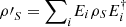 after the interaction. Then, from the previous proposition, the system of interest’s logical entropy increases. In particular, the lower bound for the logical entropy should no longer be null. This lower bound as well as an upper bound in case the joint system is pure is the concern of the next result.
Proposition 3.6 (Entropy after unitary interaction).
Assume a system S interacts with a system R through a unitary U. Also, let the joint system after the interaction be 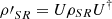 and define
  , where ρSR is the state of the joint system before the interaction and {|i〉} is an orthonormal basis of system R. Then,
![Mathematical equation: $$ {L(\rho \mathrm{\prime}}_S)\ge 2\sum_i \sum_{j < i} \left\{{tr}({B}_{{ij}}{B}_{{ij}}^{\dagger })-{Re}[{tr}({B}_{{ii}}{B}_{{jj}})]\right\}, $$](/articles/fopen/full_html/2022/01/fopen210005/fopen210005-eq58.gif) (32)
where
(32)
where  . Furthermore, if ρSR is a pure state,
 (33)
(33)
Proof. Observe that  and hence
  . As a result,
 ![Mathematical equation: $$ \begin{array}{ll}L({{\rho \prime}}_S)& =1-\sum_i \mathrm{tr}({B}_{{ii}}^2)-\sum_i \sum_{j\ne i} \mathrm{tr}({B}_{{ii}}{B}_{{jj}})\\ & =1-\sum_i \mathrm{tr}({B}_{{ii}}^2)-2\sum_i \sum_{j < i} \mathrm{Re}[\mathrm{tr}({B}_{{ii}}{B}_{{jj}})].\end{array} $$](/articles/fopen/full_html/2022/01/fopen210005/fopen210005-eq63.gif) (34)
(34)
Moreover, 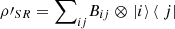 and
and 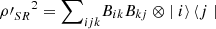 . Then, since
  ,
,  (35)
(35)
Finally, combining expressions (34) and (35), we obtain inequality (32), which completes the first part of the proof.
Now, if ρSR is a pure state, which implies that ρ′SR is also pure,  and, as a result, expression (35) becomes an equality. The left-hand side of the latter is greater or equals to L(ρ′S), as can be directly seen from (34). Therefore, we are lead to inequality (33) holds, completing the proof. □
Proposition 3.7 (Entropy of classical mixtures of quantum systems).
Let  , then
  (36)where L({pi}) is defined in (3). Moreover, the equality holds whenever the matrices ρi have orthogonal support.
Proof. To start, assume the states ρi are pure, i.e., ρi = |ψi〉〈ψi|. Then, ρ = ∑i
pi|ψi〉〈ψi|. Introducing an auxiliary system R that purifies ρ, the state of the joint system can be written as  where {|i〉} is an orthonormal basis of system R. Observe that ρ = ρS and
  (37)where
  is an orthonormal basis of S. Also, by Proposition 3.1(c),
  .
.
If ρR is measured with a PVM characterized by Pi = |i〉〈i| it holds that
  (38)
(38)
This implies that L(ρ′R) = L({pi}). Since PVMs increase the logical entropy,  (39)
(39)
Since the logical entropy of pure states vanish, the above expression proves the proposition for cases where the matrices ρi are pure states.
For the general case, let ρi = ∑ij
λij|λij〉〈λij| where the states |λ〉ij are orthonormal vectors in the subspace associated with ρi. Hence, ρ can be written as the sum of pure states ρ = ∑ij
pi
λij|λij〉〈λij| (not necessarily all orthogonal). Now, using the result for pure states we just obtained, it holds that
where the states |λ〉ij are orthonormal vectors in the subspace associated with ρi. Hence, ρ can be written as the sum of pure states ρ = ∑ij
pi
λij|λij〉〈λij| (not necessarily all orthogonal). Now, using the result for pure states we just obtained, it holds that  (40)as we wanted to show.
Finally, it follows from direct computation that the equality holds whenever the matrices ρi have orthogonal support. In fact, in this case, 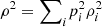 and, as a result,
 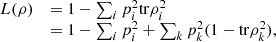 (41)which concludes the proof. □
In the next result, we prove the non-negativity of the logical divergence.
Proposition 3.8 (Klein’s inequality).
The logical divergence is always non-negative, i.e.,
 (42)
for every pair of density matrices ρ and σ, with equality holding if and only if ρ = σ.
(42)
for every pair of density matrices ρ and σ, with equality holding if and only if ρ = σ.
Proof. It follows by direct computation that  (43)
(43)
Then, recall that for any Hermitian matrix A, tr(A2) ≥ 0, with tr(A 2) = 0 if and only if A = 0. □
It should be noted that (43) defines the logical divergence as the square of the Hilbert–Schmidt norm of the difference of the two density matrices under consideration. Moreover, it can be shown that this norm coincides with a natural definition of the Hamming distance between density matrices [23].
In the next three propositions, we study the concavity of logical entropies.
Proposition 3.9 (Concavity of logical entropy).
Let ρ = ∑pi
pi
, where ρi is a density matrix for each i and 0 ≤ pi ≤ 1, such that ∑pi = 1. Moreover, set  .
.
-
If ρi have orthogonal support, then
 (44)
(44)
-
In general,
 (45)
(45)
 .
.
Proof.
-
We will demonstrate the argument on two density matrices ρ1 and ρ2 having an orthogonal support. Set ρ1 = ∑i pi|i〉〈i|

 where |i〉
 and |j〉 are two bases with orthogonal support, also set ρ = λρ1 + (1 − λ)ρ2
, where 0 < λ < 1. Now,
and |j〉 are two bases with orthogonal support, also set ρ = λρ1 + (1 − λ)ρ2
, where 0 < λ < 1. Now,
 (46)
(46)
However,
 (47)
(47)
Therefore, inequality (44) holds.
-
Consider
 so ρAB is a sum of densities with an orthogonal support. From the result in part (a) and Proposition 3.2, it follows that
 (48)
(48)
However, ρA = ρ and L(ρB) = L({pi}), which leads to  (49)proving the first part of inequality (45). To conclude the proof, we first show that
 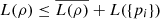 for the case where the matrices ρi are pure states, i.e., ρi = |ψi〉〈ψi|
 . For that, consider the following purification of the system:
  (50)where the vectors |i〉
 are orthonormal in some system B. Moreover, denote
  . It is clear, then, that
 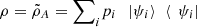 and
and 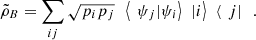 (51)
(51)
Note that the vectors |ψi〉 are not necessarily orthogonal. Measuring system B with the operators Pi = |i〉〈i|
 we obtain
 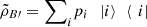 . By Proposition 3.5,
  , where we used Proposition 3.1(c) in the last step. Therefore, for ρ which is a sum of pure states, we have L(ρ) ≤ L({pi}), which is consistent with (45) since, in this case,
  .
.
Consider now the general case where ρ = ∑i
pi ρi with  (52)
(52)
Here,  are orthonormal vectors for each
  . Hence,
 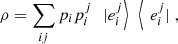 (53)where
  are pure states for every i and j. We can use the previous result for pure states to conclude that
 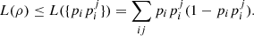 (54)
(54)
Using the fact that, for ![Mathematical equation: $ {x}_i,{x}_j\in [\mathrm{0,1}]$](/articles/fopen/full_html/2022/01/fopen210005/fopen210005-eq114.gif) ,
,  (55)we are led to
 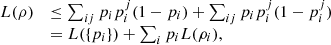 (56)where we used the orthogonality of the set of vectors
  for each
  . □
. □
Proposition 3.10 (Joint convexity of logical divergence).
The logical divergence  is jointly convex.
Proof. We start by defining ρ = λρ1 + (1 − λ)ρ2 and σ = λσ1 + (1 − λ)σ2. Then, it follows by direct computation that ![Mathematical equation: $$ \begin{array}{ll}d(\rho ||\sigma )& =\mathrm{tr}(\rho -\sigma {)}^2\\ & =\mathrm{tr}[\lambda ({\rho }_1-{\sigma }_1)+(1-\lambda )({\rho }_2-{\sigma }_2){]}^2\\ & \le \lambda \mathrm{tr}({\rho }_1-{\sigma }_1{)}^2+(1-\lambda )\mathrm{tr}({\rho }_2-{\sigma }_2{)}^2\\ & =\lambda d({\rho }_1||{\sigma }_1)+(1-\lambda )d({\rho }_2||{\sigma }_2),\end{array} $$](/articles/fopen/full_html/2022/01/fopen210005/fopen210005-eq120.gif) (57)where the inequality is due to the convexity of
(57)where the inequality is due to the convexity of  . □
. □
Proposition 3.11 (Concavity of conditional entropy).
The conditional logical entropy L(A/B) is a concave function of ρAB.
Proof. It follows direct from the relation given by (17) and Proposition 3.10. □
The next proposition states the fact that the divergence behaves as a metric. Tracing out a subspace can only reduce its value.
Proposition 3.12 (Monotonicity of logical divergence).
Let ρAB and σAB be two density matrices, then
 (58)
where b is the dimension of B.
(58)
where b is the dimension of B.
Proof. As can be seen in Chapter 11 of [16], there exist a set of unitary matrices Uj over B and a probability distribution pj such that 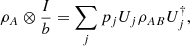 (59)for every ρAB. Then, because the logical divergence is jointly convex on both entries, we can write
  (60)
(60)
Finally, since the divergence is invariant under unitary transformations, the above sum gives d(ρAB||σAB). □
4 Quantum logical entropy of post-selected systems
We shall now propose extensions of the notion of quantum logical entropy to the class of pre- and post-selected quantum systems. Like before, we use the fact that every PVM defines a partition π in a Hilbert space given by a basis {|bi〉} associated with it since every PVM is characterized by parts Bi = |bi〉〈bi| such that ∑i
Bi = I. Suppose that a system is prepared in a state |ψ〉 and a PVM is performed. Moreover, assume that it is known that the system is later found in a state |ϕ〉 non-orthogonal to |ψ〉. In scenarios like that, with a pre-selected |ψ〉 and a post-selected |ϕ〉, the system can be represented by the generalized density matrix  (61)
(61)
The probability of measuring a result associated with  can be computed as
 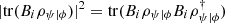 . This result is known as the ABL rule [35]. Then, in analogy with the definition of logical entropy for classical and non-post-selected quantum systems, we may define
  (62)
(62)
Since  , it holds that
 ![Mathematical equation: $$ \begin{array}{ll}{L}_{\pi }({\rho }_{\psi |\phi })& =\sum_i \mathrm{tr}|{B}_i{\rho }_{\psi |\phi }{B}_i(I-{B}_i{\rho }_{\psi |\phi }{B}_i){|}^2\\ & =|\mathrm{tr}[{\rho {\prime}}_{\psi |\phi }(I-{\rho {\prime}}_{\psi |\phi })]{|}^2,\end{array} $$](/articles/fopen/full_html/2022/01/fopen210005/fopen210005-eq130.gif) (63)where
(63)where  .
.
Differently from the case without post-selection, where a PVM-independent logical entropy could be defined by minimizing over non-degenerate PVMs, this is not possible here. The reason is that we are interested in cases where the pre- and post-selections are pure states. Then, although the minimum Lπ(ρψ|ϕ) corresponds to the case where  , it also corresponds to the null function. This is the case because in such scenarios the intermediate PVM is associated with an orthonormal basis that contains either |ψ〉 or |ϕ〉. As a result, these PVMs allow us to see ρψ|ϕ as a partition with a single part.
Observe that, by construction, the logical entropy for post-selected systems is always positive. This fact contrasts with a generalization of the von Neumann entropy proposed in [36], which can assume negative values for some post-selections.
Another approach for this problem employs directly the notion of weak values [37], which has been shown to be very constructive in the study of pre- and post-selected systems [38–50]. This approach consists of replacing the intermediate PVM by the inference of the weak values of orthogonal projectors associated with a specific PVM. Given a pre-selection |ψ〉, a post-selection |ϕ〉, and a PVM characterized by parts (projectors) Bi, the weak value associated with each operator Bi is defined as tr(Bi ρψ|ϕ). Since ∑itr(Bi
ρψ|ϕ), the weak values of this set of projectors can be seen as a quasi-probability distribution. It is possible, then, to use these quasi-probabilities to construct a weak logical entropy for post-selected quantum systems, which gives ![Mathematical equation: $$ \begin{array}{cc}{L}_{\pi }^w({\rho }_{\psi |\phi })& \equiv \sum_i \mathrm{tr}({B}_i{\rho }_{\psi |\phi })\mathrm{tr}[(I-{B}_i){\rho }_{\psi |\phi }]\\ & =\sum_i \mathrm{tr}({B}_i{\rho }_{\psi |\phi })[1-\mathrm{tr}({B}_i{\rho }_{\psi |\phi })]\\ & =\mathrm{tr}\left[{{\rho }^\mathrm{\prime}}_{\psi |\phi }\left(I-{{\rho }^\mathrm{\prime}}_{\psi |\phi }\right)\right].\end{array} $$](/articles/fopen/full_html/2022/01/fopen210005/fopen210005-eq133.gif) (64)
(64)
Here, again, a PVM-independent logical entropy cannot be defined. However, just like the extension of the von Neumman entropy to post-selected systems [36], the weak logical entropy can be negative. Even further, it may be complex-valued.
While the operational meaning of Lπ (ρψ|ϕ) is clear, it is not straightforward to interpret  . One of the reasons is that weak values are associated with weak measurements, and weak measurements do not divide the Hilbert space into disjoints parts. In fact, weak measurements can be seen as an interpolation between the identity map, which does not disturb the system but does not provide any information about it, and the associated PVM map, which provides maximum information about the system [51]. The weaker the measurement, the bigger the contribution of the identity map in this interpolation. It is clear from the discussion in this work that, while the PVM introduces partitions to the Hilbert space, the indetity map does not make distinction between any part. This fact in itself can be seen as the reason we end up with a quasiprobability (and not a probability) distribution.
However, consider the following game: A system is prepared in a state |ψ〉. Later, a weak measurement of one of the blocks Bi of a given PVM is performed. The system is then post-selected in the state |ϕ〉. If this process is repeated and the PVM is composed by n blocks, then the probability that the weak measurement of a different block is performed is simply (n − 1)/n. However, suppose that, instead, we wanted to refer to the obtained weak value as the quasiprobability associated with each block. In this case, keeping an algebraic analogy to the classical logical entropy defined in (2) and the PVM-dependent quantum logical entropy defined in (5), we obtain the weak logical entropy  .
.
Interestingly, even though the logical and the weak logical entropies of post-selected systems are associated with different operational meanings, it should be noted that 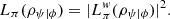 (65)
(65)
Thus, in this sense, the weak logical entropy is mathematically more fundamental than the logical entropy of post-selected systems first introduced in this section.
5 Discussion
In this work we presented a new approach to the introduction of quantum logical entropy that maintains a clear connection to the notion of partition. As we discussed, the PVM-independent definition of this entropy is equivalent to other already known quantities. However, the perspective of partitions that comes with its introduction may bring new insights into its use in the study of quantum systems within different scenarios. Furthermore, it may lead to the discovery of new implications for the logical structure, uncertainty, and information processing associated with quantum systems.
In fact, the properties of logical entropies proved here may be relevant to quantum information science and technology as well as other areas of quantum mechanics, as already shown, e.g., in [11, 52–55]. In particular, a special case of Proposition 3.6 concerns quantum systems in the presence of noise. In this case, the logical entropy of the system of interest after its interaction with the noise is bounded by correlations between this system and its environment. This scenario, including an example of amplitude damping, was considered in [56]. Moreover, since the logical entropy is a measure of distinction, it seems natural to use it in the investigation of channel capacity in terms of distinctions. We expect that the language of quantum distinctions may simplify the proofs of channel properties. It would be also interesting to examine the use of logical entropy in the context of entanglement quantification in discrete/continuous systems.
Notably, while some of the properties of logical entropies are similar to the ones held by the more widely studied von Neumann entropy, many of them also evidence major differences. It stands out, for instance, that the logical entropy does not fulfill the strong subadditivity property. Even though it still satisfies subadditive properties, as stated in Propositions 3.2 and 3.3, the “breakdown” of strong additivity implies an unmistakable departure from the von Neumann entropy. The lack of this property might at first appear somewhat troublesome. However, it may also place the quantum logical entropy as a fundamental player in various special scenarios, e.g., when discussing the breakdown of subadditivity in black holes [57].
Finally, we briefly extended the notion of logical entropy to post-selected quantum systems in two ways. In the first, there exists a clear operational meaning associated with the logical entropy. In the second (weak logical entropy), there exists only a loose connection with experimental procedures associated with weak measurements. It would be important to study better the significance of the latter. Furthermore, properties of these logical entropies need yet to be investigated. Also, a relation between both definitions can be established as seen in (65), where the square of the magnitude of the weak logical entropy gives the logical entropy of post-selected systems. This raises a question about the phase of the weak logical entropy. While we could not find a direct meaning to it, it seems to us that this problem deserves further analysis.
Conflict of interest
The authors declare that they have no conflict of interest.
Acknowledgments
We thank D. Ellerman and Y. Neuman for many discussions on the topic as well as their helpful comments. We are also thankful to T. Landsberger and J. Kupferman for helpful feedback regarding a previous version of this manuscript. E.C. was supported by Grant No. FQXi-RFP-CPW-2006 from the Foundational Questions Institute and Fetzer Franklin Fund, a donor advised fund of Silicon Valley Community Foundation, the Israel Innovation Authority under Projects No. 70002 and No. 73795, the Quantum Science and Technology Program of the Israeli Council of Higher Education, and the Pazy Foundation.
References
- Brukner Č, Zeilinger A (1999), Operationally invariant information in quantum measurements. Phys Rev Lett 83, 3354. [CrossRef] [Google Scholar]
- Brukner Č, Zeilinger A (2001), Conceptual inadequacy of the Shannon information in quantum measurements. Phys Rev A 63, 022113. [CrossRef] [Google Scholar]
- Giraldi F, Grigolini P (2001), Quantum entanglement and entropy. Phys Rev A 64, 032310. [CrossRef] [Google Scholar]
- Cover TM, Thomas JA (2006), Elements of Information Theory, 2nd edn., Wiley, Hoboken, New Jersey. [Google Scholar]
- Ellerman D (2013), Information as distinctions: New foundations for information theory, arXiv:1301.5607. [Google Scholar]
- Tsallis C (1988), Possible generalization of Boltzmann-Gibbs statistics. J Stat Phys 52, 479. [CrossRef] [Google Scholar]
- Manfredi G, Feix MR (2000), Entropy and Wigner functions. Phys Rev E 62, 4665. [CrossRef] [PubMed] [Google Scholar]
- Ellerman D (2013), An introduction to logical entropy and its relation to Shannon entropy. Int J Semant Comput 7, 121. [CrossRef] [Google Scholar]
- Ellerman D (2014), An introduction to partition logic. Log J IGPL 22, 94. [CrossRef] [Google Scholar]
- Tamir B, Cohen E (2014), Logical entropy for quantum states, arXiv:1412.0616. [Google Scholar]
- Tamir B, Cohen E (2015), A Holevo-type bound for a Hilbert Schmidt distance measure. J Quantum Inf Sci 5, 127. [CrossRef] [Google Scholar]
- Gini C (1912), Variabilità e Mutabilità: Contributo allo Studio delle Distribuzioni e delle Relazioni Statistiche. [Fasc. I.]. Studi economico-giuridici pubblicati per cura della facoltà di Giurisprudenza della R. Università di Cagliari. Tipogr. di P. Cuppini. [Google Scholar]
- Rejewski M (1981), How Polish mathematicians broke the Enigma Cipher. Ann Hist Comput 3, 213. [CrossRef] [Google Scholar]
- Patil GP, Taillie C (1982), Diversity as a concept and its measurement. J Am Stat Assoc 77, 548. [CrossRef] [Google Scholar]
- Good IJ (1982), Comment: Diversity as a concept and its measurement. J Am Stat Assoc 77, 561. [Google Scholar]
- Nielsen MA, Chuang IL (2010), Quantum information and quantum computation, University Press, Cambridge. [CrossRef] [Google Scholar]
- Ellerman D (2014), Partitions and objective indefiniteness in quantum mechanics, arXiv:1401.2421. [Google Scholar]
- Ellerman D (2016), On classical and quantum logical entropy. Available at SSRN 2770162. https://doi.org/10.2139/ssrn.2770162 . [Google Scholar]
- Ellerman D (2016), On classical and quantum logical entropy: The analysis of measurement, arXiv:1604.04985. [Google Scholar]
- Ellerman D (2017), New logical foundations for quantum information theory: Introduction to quantum logical information theory, arXiv:1707.04728. [Google Scholar]
- Ellerman D (2017), Introduction to quantum logical information theory, Available at SSRN 3003279. https://doi.org/10.2139/ssrn.3003279 . [Google Scholar]
- Ellerman D (2018), Introduction to quantum logical information theory: Talk. EPJ Web Conf 182, 02039. [CrossRef] [EDP Sciences] [Google Scholar]
- Ellerman D (2018), Logical entropy: Introduction to classical and quantum logical information theory. Entropy 20, 679. [CrossRef] [Google Scholar]
- Ellerman D (2016), The quantum logic of direct-sum decompositions. Available at SSRN 2770163. https://doi.org/10.2139/ssrn.2770163. [Google Scholar]
- Ellerman D (2018), The quantum logic of direct-sum decompositions: the dual to the quantum logic of subspaces. Log J IGPL 26, 1. [CrossRef] [Google Scholar]
- Auletta G, Fortunato M, Parisi G (2009), Quantum mechanics, Cambridge University Press, New York. [Google Scholar]
- Lüders G (1950), Über die Zustandsänderung durch den Meßprozeß. Ann Phys 443, 322. [CrossRef] [Google Scholar]
- von Neumann J (1932), Mathematische Grundlagen der Quantenmechanik, Springer, Berlin. [Google Scholar]
- Jaeger G (2007), Quantum information: an overview, Springer, New York. [Google Scholar]
- Coles PJ (2011), Non-negative discord strengthens the subadditivity of quantum entropy functions, arXiv:1101.1717. [Google Scholar]
- Audenaert KMR (2007), Subadditivity of q-entropies for q > 1. J Math Phys 48, 083507. [CrossRef] [Google Scholar]
- Streltsov A, Kampermann H, Wolk S, Gessner M, Brub D (2018), Maximal coherence and the resource theory of purity. New J Phys 20, 053058. [CrossRef] [Google Scholar]
- Uhlmann A (1970), On the Shannon entropy and related functionals on convex sets. Rep Math Phys 1, 147. [CrossRef] [Google Scholar]
- Nielsen MA (2002), An introduction to majorization and its applications to quantum mechanics (Lecture Notes), Department of Physics, University of Queensland, Australia. [Google Scholar]
- Aharonov Y, Bergmann PG, Lebowitz JL (1964), Time symmetry in the quantum process of measurement. Phys Rev 134, B1410. [CrossRef] [Google Scholar]
- Salek S, Schubert R, Wiesner K (2014), Negative conditional entropy of postselected states. Phys Rev A 90, 022116. [CrossRef] [Google Scholar]
- Aharonov Y, Albert DZ, Vaidman L (1988), How the result of a measurement of a component of the spin of a spin-1/2 particle can turn out to be 100. Phys Rev Lett 60, 1351. [CrossRef] [PubMed] [Google Scholar]
- Dixon PB, Starling DJ, Jordan AN, Howell JC (2009), Ultrasensitive beam deflection measurement via interferometric weak value amplification. Phys Rev Lett 102, 173601. [CrossRef] [PubMed] [Google Scholar]
- Jacobs K (2009), Second law of thermodynamics and quantum feedback control: Maxwell’s demon with weak measurements. Phys Rev A 80, 012322. [CrossRef] [Google Scholar]
- Turner MD, Hagedorn CA, Schlamminger S, Gundlach JH (2011), Picoradian deflection measurement with an interferometric quasi-autocollimator using weak value amplification. Opt Lett 36, 1479. [CrossRef] [PubMed] [Google Scholar]
- Aharonov Y, Cohen E, Elitzur AC (2014), Foundations and applications of weak quantum measurements. Phys Rev A 89, 052105. [CrossRef] [Google Scholar]
- Dressel J, Malik M, Miatto FM, Jordan AN, Boyd RW (2014), Colloquium: Understanding quantum weak values: Basics and applications. Rev Mod Phys 86, 307. [CrossRef] [Google Scholar]
- Alves GB, Escher BM, de Matos Filho RL, Zagury N, Davidovich L (2015), Weak-value amplification as an optimal metrological protocol. Phys Rev A 91, 062107. [CrossRef] [Google Scholar]
- Cortez L, Chantasri A, Garca-Pintos LP, Dressel J, Jordan AN (2017), Rapid estimation of drifting parameters in continuously measured quantum systems. Phys Rev A 95, 012314. [CrossRef] [Google Scholar]
- Kim Y, Kim Y-S, Lee S-Y, Han S-W, Moon S, Kim Y-H, Cho Y-W (2018), Direct quantum process tomography via measuring sequential weak values of incompatible observables. Nat Commun 9, 192. [CrossRef] [PubMed] [Google Scholar]
- Naghiloo M, Alonso JJ, Romito A, Lutz E, Murch KW (2018), Information gain and loss for a quantum Maxwell’s demon. Phys Rev Lett 121, 030604. [CrossRef] [PubMed] [Google Scholar]
- Hu M-J, Zhou Z-Y, Hu X-M, Li C-F, Guo G-C, Zhang Y-S (2018), Observation of non-locality sharing among three observers with one entangled pair via optimal weak measurement. npj Quantum Inf 4, 63. [CrossRef] [Google Scholar]
- Pfender M, Wang P, Sumiya H, Onoda S, Yang W, Dasari DBR, Neumann P, Pan X-Y, Isoya J, Liu R-B, Wrachtrup J (2019), High-resolution spectroscopy of single nuclear spins via sequential weak measurements. Nat Commun 10, 594. [CrossRef] [PubMed] [Google Scholar]
- Cujia KS, Boss JM, Herb K, Zopes J, Degen CL (2019), Tracking the precession of single nuclear spins by weak measurements. Nature 571, 230. [CrossRef] [PubMed] [Google Scholar]
- Paiva IL, Aharonov Y, Tollaksen J, Waegell M (2021), Aharonov-Bohm effect with an effective complex-valued vector potential, arXiv:2101.11914. [Google Scholar]
- Dieguez PR, Angelo RM (2018), Information-reality complementarity: The role of measurements and quantum reference frames. Phys. Rev. A 97, 022107. [CrossRef] [Google Scholar]
- Zurek WH, Habib S, Paz JP (1993), Coherent states via decoherence. Phys Rev Lett 70, 1187. [CrossRef] [PubMed] [Google Scholar]
- Buscemi F, Bordone P, Bertoni A (2007), Linear entropy as an entanglement measure in two-fermion systems. Phys Rev A 75, 032301. [CrossRef] [Google Scholar]
- Nayak AS, Devi ARU, Rajagopal AK, et al. (2017), Biseparability of noisy pseudopure, W and GHZ states using conditional quantum relative Tsallis entropy. Quantum Inf Process 16, 51. [CrossRef] [Google Scholar]
- Khordad R, Sedehi HRR (2017), Application of non-extensive entropy to study of decoherence of RbCl quantum dot qubit: Tsallis entropy. Superlattices Microstruct 101, 559. [CrossRef] [Google Scholar]
- Tamir B (2017), Tsallis entropy is natural in the formulation of quantum noise, arXiv:1702.07864. [Google Scholar]
- Almheiri A, Marolf D, Polchinski J, Sully J (2013), Black holes: complementarity or firewalls? J High Energy Phys 2, 62. [CrossRef] [Google Scholar]
Cite this article as: Tamir B, Paiva I, Schwartzman-Nowik Z & Cohen E 2022. Quantum logical entropy: fundamentals and general properties. 4open, 5, 2.
All Figures
|
Figure 1 Pictorial representation of a set with a partition and its distinction. (a) A set U with six elements ui is divided in a partition π with three blocks (green areas). (b) The set U × U has each of its points characterized by a square in a 2D mesh. Points that belong to dit(π), i.e., pairs whose components belong to different blocks are colored in green. |
| In the text | |
|
Figure 2 Representation of the probability distribution used in the definition of quantum logical entropy. Any state ρ, together with a partition characterized by a PVM, which is associated with an orthonormal basis in the corresponding Hilbert space, defines a probability distribution. This is the case even in case of coarse (i.e., degenerate) PVMs, as illustrated by the yellow partition. These distributions allow the introduction of (PVM-dependent) logical entropies for quantum systems. |
| In the text | |