| Issue |
4open
Volume 2, 2019
Difference & Differential Equations and Applications
|
|
|---|---|---|
| Article Number | 26 | |
| Number of page(s) | 12 | |
| Section | Mathematics - Applied Mathematics | |
| DOI | https://doi.org/10.1051/fopen/2019015 | |
| Published online | 11 July 2019 | |
Research Article
Mathematical models for optimising bi-enzyme biosensors
1
School of Hospitality Management and Tourism, Technological University Dublin, 40–45 Mountjoy Square, Dublin 1, Ireland
2
School of Computer Science, Technological University Dublin, Kevin Street, Dublin 8, Ireland
* Corresponding author: This email address is being protected from spambots. You need JavaScript enabled to view it.
Received:
28
December
2018
Accepted:
4
May
2019
Abstract
From our previous work we have seen examples of problems where including diffusion of a reactant into the model only affects the transient behaviour of the system but has no effect on the final steady states of its concentration. The equilibrium values are the only piece of information required for the solution of our experimental problem and in such situations it is important to identify the conditions under which a complex partial differential equations model can be replaced with a simpler one. The aim of this study is to find the optimal ratio of the two enzymes involved with a bi-enzyme electrode based on a flow injection analysis. Three mathematical models was constructed each neglect different aspects of the biosensor functionality. A detailed comparison of the models was carried out, base on various physical conditions recommendations of the best modelling strategy were given.
Key words: Biosensors / Cascade reactions / Equilibrium / Steady-state
© Q. Wang & Y. Liu, Published by EDP Sciences, 2019
 This is an Open Access article distributed under the terms of the Creative Commons Attribution License (http://creativecommons.org/licenses/by/4.0/), which permits unrestricted use, distribution, and reproduction in any medium, provided the original work is properly cited.
Introduction
In order to build a platform for biosensers based on a bi-enzyme electrode a research group at Dublin City University in Ireland have conducted a series of experiments which motivated this reseach work (refer to [1, 2] for details). The biosensor system investigated in this paper consists of two enzymes: glucose oxidase (GOX) and horseradish peroxidase (HRP), they are both immobilised onto an electrode modified with a conducting polymer. The two enzymes have very different kinetic characteristics, the performance of the system will depend on the optimal ratio of the two enzymes. A cascade reaction takes place at the electrode, GOX catalyses the oxidation reaction of glucose to gluconic acid, with production of H2O2. HRP is oxidised by hydrogen peroxide and then subsequently reduced by electrons provided by the electrode, which can be summarised as:
Modelling strategies
A number of simplifying assumptions are made in order to carry out mathematical modelling for these reactions (refer to [3] for details). The standard Michaelis–Menten equation (1) was used to model this biochemical reaction:
 (1)where E
1 represents glucose oxidase, E
2 represents horseradish peroxidase, S
1 and S
2 represent the two substrates: glucose and hydrogen peroxide, C
1 and C
2 represent the two complexes and P represents the final product. All the k values denote the reactions rate, which are all constant.
(1)where E
1 represents glucose oxidase, E
2 represents horseradish peroxidase, S
1 and S
2 represent the two substrates: glucose and hydrogen peroxide, C
1 and C
2 represent the two complexes and P represents the final product. All the k values denote the reactions rate, which are all constant.
Three models of varying complexity for analysing this optimisation problem were discussed. Analytical solutions were presented with a view to expressing the steady-state current as a function of the ratio ζ of the two immobilised enzymes and thus finding its maximum value.
The first model, the “comprehensive model” assumes that the two substrates, S 1 and S 2, are free to diffuse in the solution and consists of two diffusion equations with the relevant nonlinear reaction-type boundary conditions. This model was proposed and solved numerically in [1]. We then jump to the other extreme and ignore all transport phenomena basically reducing the whole problem to the one-point kinetics of the cascade reaction in the second model, the “simplified model”. This leads to a system of ordinary differential equations which is analysed using a combination of dynamical systems methods, perturbation techniques and numerical simulations. This model was also studied previously in Refs. [2, 3]. Finally, the third model, the “intermediate model” is proposed here for the first time and is a compromise between the two situations discussed above, where we allow one substrate (hydrogen peroxide) to diffuse but assume the other substrate (glucose) is only present at the electrode, in comparison with the first model, we obtain a much simpler system.
It is perhaps instructive to give some motivations regarding the choice of these three models and discuss expectations. We expect the diffusion of the first substrate S 1 to the electrode will have no effect on the equilibrium state except by increasing the time it takes to achieve it. So we expect there will be little difference between the first and third model. On the other hand, neglecting the diffusion of the second substrate S 2 (hydrogen peroxide) in the second model is potentially more serious as this assumes that all S 2 generated in the first reaction is immediately available for the second reaction and this could affect the size of the final steady states.
The comprehensive model
This section reviews the model introduced in [1] (where both substrates diffuse). An additional steady-state analysis of the partial differential equations is also presented.
Review of the comprehensive model
In this model, the cascade scheme (1) is modelled by a system of partial differential equations and boundary conditions representing convective and diffusive transport of the two substrates, glucose and hydrogen peroxide, as well as the reaction kinetics of the bi-enzyme electrode. For simplicity, the convective transport is not explicitly modelled and the flow injection is only reflected in the boundary conditions imposed at the top of the diffusion domain, 0 ≤ x ≤ L. We have also assumed that diffusion is one-dimensional and x measures distance from the electrode.
In what follows, we denote the concentrations of all the chemical species mentioned in the cascade scheme (1) by their corresponding lower case letters (e.g., s 1 = [S 1], etc.). The two substrates satisfy the following diffusion equations:
 where D
1 and D
2 denotes the coefficients of diffusion. The top boundary conditions were formed based on the fact that the first substrate S
1 is continuously injected into the solution at a constant speed, and the second substrate S
2 is flushed away constantly, where,
where D
1 and D
2 denotes the coefficients of diffusion. The top boundary conditions were formed based on the fact that the first substrate S
1 is continuously injected into the solution at a constant speed, and the second substrate S
2 is flushed away constantly, where,
 The bottom boundary conditions are:
 together with,
The initial conditions are:

 where
where  ,
,  and s
0 are constants. We let,
and s
0 are constants. We let,
 which implies,
 in which e represents the total amount of e
1 and e
2 consumed in the biochemical reaction, it is a constant parameter which can be measured experimentally.
in which e represents the total amount of e
1 and e
2 consumed in the biochemical reaction, it is a constant parameter which can be measured experimentally.
The system is non-dimensionalised by the variables as shown below:
 where t
0 = 1/(k
1
s
0). We then obtain the non-dimensional system,
where t
0 = 1/(k
1
s
0). We then obtain the non-dimensional system,
 (2)where the bars were dropped for convenience. An extensive numerical analysis of this system was presented in [1] where the behaviour of the enzyme ratio ζ was studied for different values of the system parameters. The time evolution of
  , which was taken as a measure of the amperometric signal, was calculated and the steady state value,
  , was recorded as the current value and used for future parameter iterations. Note that the dimensional value of the current is,
 (3)hence,
  can be regarded as a good measure of the amperometric signal, which should not depend on the choice of non-dimensionalisation used in the model.
Steady-state analysis
This part of the paper analyse system (2) as t → ∞. At equilibrium, equation (2a) gives,
 which means,
 (4)then integrating equation (4) twice with respect to x, we get,
 (5)Similarly, from equation (2b), we obtain,
 (6)where
  ,
,  denote the equilibrium values of s
1(x, t), s
2(x, t) respectively, and A, B, C, D are constants of integration.
denote the equilibrium values of s
1(x, t), s
2(x, t) respectively, and A, B, C, D are constants of integration.
Equation (2c) together with equation (5) gives,
 similarly equation (2d) together with equation (6) gives,
 Thus, at x = 0, the system (2) can be reduced to,
 (7)Here, we have a system of four equations with four unknowns B, D,
  and
and  , we then reduce the system to two equations in terms of
  and
and  , which denote the equilibrium values of c
1(t), c
2(t) respectively.
, which denote the equilibrium values of c
1(t), c
2(t) respectively.
 (8)System (8) can be easily solved to give explicit formulas for
  and
and  where,
 (9)
(9)
 (10)Note that the smaller solution is selected in both these quadratic equations, as we need,
 We then plot the current,
  , as a function of ζ by using MAPLE in Figure 1. We note that, as we chose k
2 = k
4, the optimal ratio ζ* approaches one for large glucose concentrations. Figure 2 shows the current as a function of ζ when the ratio k
4/k
2 is varied.
, as a function of ζ by using MAPLE in Figure 1. We note that, as we chose k
2 = k
4, the optimal ratio ζ* approaches one for large glucose concentrations. Figure 2 shows the current as a function of ζ when the ratio k
4/k
2 is varied.
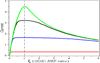 |
Figure 1 Dependence of current on ζ. s 0 = 1 (red), 5 (blue), 10 (black) and 20 (green) mM, k 1 = 102, k −1 = 10−1, k 2 = 10, k 3 = 102, k −3 = 10−1, k 4 = 10, e 0 = 10−5, l = 2 × 10⁻⁴, D 1 = 6.7 × 10⁻¹⁰ and D 2 = 8.8 × 10⁻¹⁰. |
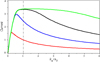 |
Figure 2 Dependence of current on ζ. k 4/k 2 = 0.2 (red), 0.5 (blue), 1 (black) and 2 (green), k 1 = 102, k −1 = 10−1, k 2 = 10, k 3 = 102, k −3 = 10−1, k 4 = 10, e 0 = 10−5, l = 2 × 10⁻⁴, D 1 = 6.7 × 10⁻¹⁰ and D 2 = 8.8 × 10⁻¹⁰. |
Simplified model
This section analyses the simple, one-point model of the cascade reaction which was introduced in [2]. A very detailed analysis of the model is presented in [3], the behaviour of the system for different ζ is discussed in here.
Review of the simple model
The following non-dimentional system of ordinary differential equations were constructed for the one-point model based on the fact that the substrates do not diffuse in the biochemical reaction:
 (11)We can further simplify system (11) as follows since the first substrate glucose is supplied constantly at the electrode,
 with initial conditions c
1 (0) = 0, c
2 (0) = 0 and s
2 (0) = 0, where,
with initial conditions c
1 (0) = 0, c
2 (0) = 0 and s
2 (0) = 0, where,
The global behaviour of system (12) is analysed by using the slow-fast dynamics, slow invariant manifold and the dynamical systems analysis (refer to [3] for details), we concluded system (12) has the following long term behaviours,
 (13)
(13)
 (14)
(14)
 (15)where,
 (16)
(16)
 (17)
(17)
 (18)
(18)
 (19)From these results, we can see that when ζ < ζ*, the initial amount of glucose oxidase is less than the initial amount of horseradish peroxidase. This leads to the amount of s
2 produced from the first reaction is all consummed somehow in the second reaction and eventually an equilibrium state can be reached; and when ζ ≥ ζ*, the initial amount of glucose oxidase is greater than the initial amount of horseradish peroxidase. The production rate is greater than the comsumption rate of s
2, so the concentration of s
2 will increase indefinitely.
(19)From these results, we can see that when ζ < ζ*, the initial amount of glucose oxidase is less than the initial amount of horseradish peroxidase. This leads to the amount of s
2 produced from the first reaction is all consummed somehow in the second reaction and eventually an equilibrium state can be reached; and when ζ ≥ ζ*, the initial amount of glucose oxidase is greater than the initial amount of horseradish peroxidase. The production rate is greater than the comsumption rate of s
2, so the concentration of s
2 will increase indefinitely.
We plot the steady state current, k 4 c 2(∞), as a function of ζ for different values of s 0 (Fig. 3) and k 4/k 2 (Fig. 4). In Figure 3 the curves overlay for ζ values ranging from 1 to 6, and in Figure 4 the curves overlay for ζ values ranging from 0 to 1, also note that from equation (14a) and (14b), that the optimal enzymes ratio is given by,
 as c
2(∞) achieves its maximum value of 1/(1 + ζ*) when ζ = ζ*. Therefore, we are able to obtain an explicit formula which gives the optimal value of ζ in terms of the system parameters. Note the agreement between the results as shown in Figures 3 and 4 and the model in the previous section.
as c
2(∞) achieves its maximum value of 1/(1 + ζ*) when ζ = ζ*. Therefore, we are able to obtain an explicit formula which gives the optimal value of ζ in terms of the system parameters. Note the agreement between the results as shown in Figures 3 and 4 and the model in the previous section.
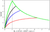 |
Figure 3 Dependence of current on ζ. s 0 = 0.03 (red), 0.09 (blue), 0.2 (black) and 5 (green) mM, k 1 = 102, k −1 = 10−1, k 2 = 10 and k 4 = 10. |
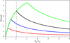 |
Figure 4 Dependence of current on ζ. k 4/k 2 = 0.2 (red), 0.5 (blue), 1 (black) and 2 (green), k 1 = 102, k −1 = 10−1, k 2 = 10 and k 4 = 10. |
Intermediate model
In this model, we assume the glucose (s 1) does not diffuse but is present only at the electrode boundary point, and in addition it is constant, i.e., s 1(t) = s 0. (In other words, s 1 is supplied continuously at the reaction site.) The second substrate is free to diffuse throughout the domain at all times during the experiment, which is reflected by the following diffusion equation,
At the top layer and the electrode, we have the boundary conditions,

 together with,
The initial conditions are:
 and the conservation laws are:
The system is non-dimensionalised by using the variables below,
 where t
0 = 1/(k
1
s
0); we then obtain the non-dimensional system,
where t
0 = 1/(k
1
s
0); we then obtain the non-dimensional system,
 (20)with non-dimensional initial conditions,
 and conservation laws,
 where,
We now carry out a steady-state analysis of system (20). At equilibrium,
 which gives,
 (21)
(21)
Then by integrating (21) twice, we obtain,
 which gives,
 (22)where
  denotes the equilibrium value of s
2(x, t), A and B are constants of integration. Also, from equation (20c), we obtain A = −B and this condition together with equation (22) yields,
denotes the equilibrium value of s
2(x, t), A and B are constants of integration. Also, from equation (20c), we obtain A = −B and this condition together with equation (22) yields,
 which gives,
 (23)From equation (20e), we obtain
 and, from equation (20f), we obtain,
 Also, from equations (20d) and (23), we get,
 which gives,
 from which, B can be easily obtained as a function of ζ, i.e., B(ζ) (Note that since the above quadratic equation has two real roots of different signs, we choose the positive root). Thus, the equilibrium value for the current is,
 Figure 5 shows the plot of current (
 ) on ζ for various values of s
0; if we vary k4/k
2 instead, we obtain the graphs in Figure 6.
) on ζ for various values of s
0; if we vary k4/k
2 instead, we obtain the graphs in Figure 6.
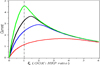 |
Figure 5 Dependence of current on ζ. s 0 = 0.03 (red), 0.09 (blue), 0.2 (black) and 5 (green), k 1 = 102, k −1 = 10−1, k 2 = 10, k 3 = 102, k −3 = 10−1, k 4 = 10, e 0 = 10−5, l = 2 × 10⁻⁴ and D 1 = 6.7 × 10⁻¹⁰. |
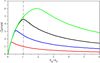 |
Figure 6 Dependence of current on ζ. k 4/k 2 = 0.2 (red), 0.5 (blue), 1 (black) and 2 (green), k 1 = 102, k −1 = 10−1, k 2 = 10, k 3 = 102, k −3 = 10−1, k 4 = 10, e 0 = 10−5, l = 2 × 10⁻⁴ and D 1 = 6.7 × 10⁻¹⁰. |
Summary and comparisons
The work presented here shows the study of a bi-enzyme electrode based on a flow injection analysis, with the aim of finding the optimal ratio of the two enzymes involved. Three different mathematical models were considered: the “comprehensive model” (where we include the diffusion effects of the two substrates: glucose and hydrogen peroxide), the “simplified model” (which concentrated on the kinetics of the two reactions and no transport was taken into account) and the “intermediate model” (which only considered the diffusion of the substrate hydrogen peroxide). As the simplified model consisted of a system of ordinary differential equations, we were able to present a detailed analytical study of its solutions (including an exact formula for the optimal ratio of the two enzymes), unlike in the other two models where the results were mostly numerical.
The dependence of the biosensor response (i.e., the measured amperometric current) as a function of ζ, the ratio of the two enzymes, is again plotted in Figure 7, for different values of the glucose concentration and, in Figure 8, for different values of k 4/k 2. Figures 7a and 8a are plotted based on the experimental data from [1].
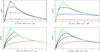 |
Figure 7 Dependence of current on ζ for different initial concentrations of s 0. Steady-state analysis of (a) and (b) comprehensive model, (c) simplified model, and (d) intermediate model. |
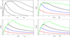 |
Figure 8 Dependence of current on ζ for different values of k 4/k 2. Steady-state analysis of (a) and (b) comprehensive model, (c) simplified model, and (d) intermediate model. |
To facilitate the comparison of the three models, we then plot the optimal ζ value (the value which maximises the current) as a function of the glucose concentration. The four resulting curves are as shown in Figure 9.
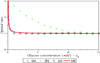 |
Figure 9 Dependence of optimal enzyme ratio on s 0 (glucose oxidase concentration). (a) Steady-state analysis of intermediate model, (b) numerical analysis of comprehensive model, (c) steady-state analysis of comprehensive model, and (d) steady-state analysis of simplified model. |
We note that the simple model and the intermediate model give identical results for the optimal enzyme ratio for all values of initial glucose concentration. The values predicted by the comprehensive model are quite different at low glucose concentrations but, again, identical at high glucose concentrations. Note that, at high glucose concentration, the optimal enzyme ratio approaches the same value regardless of the model used (This value is ζ* = 1 in our graph, as a consequence of choosing k 2 = k 4.). The fact that a given optimal enzyme ratio is achieved at a higher value of glucose concentration in the comprehensive model is quite obvious, since in that model the glucose is diffusing from a distant place (unlike in the other two models where s 0 represents the glucose concentration at the reaction site). Also, at high glucose concentrations, we expect both enzymes to be saturated with the corresponding substrates (i.e., working at maximum capacity) and so increasing the amount of glucose will not make any difference to the biosensor performance. The three models will give the same result in this regime as the transport effects only affect the availability of substrates at the reaction site.
Next, we studied the dependence of the optimal enzyme ratio on a different parameter associated with our chemical system, namely k 4/k 2 which represents the ratio of the catalytic turnover numbers for the two consecutive reactions. The optimal ratio ζ was plotted against k 4/k 2 for the three models and the resulting graphs are shown in Figure 10. Note that, the simple model predicts a linear relationship between ζ* and k 4/k 2, as illustrated by equation (19). The three models seem to give identical results at low values of k 4/k 2, but diverge when the second reaction becomes much faster than the first.
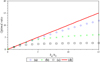 |
Figure 10 Dependence of optimal enzyme ratio on k 4/k 2 ratio. (a) Steady-state analysis of intermediate model, (b) numerical analysis of comprehensive model, (c) steady-state analysis of comprehensive model, and (d) steady-state analysis of simplified model. |
In conclusion, parameter regimes which are characterised by high glucose concentrations and low values of k 4/k 2 seem relatively indifferent to the modelling strategy used and so we would recommend the simple model, which is the easiest to analyse. For all the other parameter regions, further understanding of the behaviour of the system is required and our results so far seem to imply that we need to investigate the relationship between diffusion rates and the speeds of the two reactions. An asymptotic analysis based on these parameters will form the subject of a future study.
References
- Mackey D, Killard AJ, Ambrosi A, Smyth MR (2007), Optimizing the ratio of horseradish peroxidase and glucose oxidase on a bienzyme electrode: Comparison of a theoretical and experimental approach. Sens Actuators B122, 395–402. [CrossRef] [Google Scholar]
- Mackey D, Killard AJ (2008), Optimising design parameters of enzyme-channelling biosensors, in: Mattheij R, et al. (Eds.), Progress in Industrial Mathematics at ECMI 2006, Springer, Berlin, Heidelberg, 853–857. [CrossRef] [Google Scholar]
- Wang Q, Liu Y (2017), Mathematical model for optimising bi-enzyme biosensors, in: Differential and Difference Equations with Applications, Springer, Cham, 595–615. [Google Scholar]
Cite this article as: Wang Q & Liu Y 2019. Mathematical models for optimising bi-enzyme biosensors. 4open, 2, 26.
All Figures
|
Figure 1 Dependence of current on ζ. s 0 = 1 (red), 5 (blue), 10 (black) and 20 (green) mM, k 1 = 102, k −1 = 10−1, k 2 = 10, k 3 = 102, k −3 = 10−1, k 4 = 10, e 0 = 10−5, l = 2 × 10⁻⁴, D 1 = 6.7 × 10⁻¹⁰ and D 2 = 8.8 × 10⁻¹⁰. |
| In the text | |
|
Figure 2 Dependence of current on ζ. k 4/k 2 = 0.2 (red), 0.5 (blue), 1 (black) and 2 (green), k 1 = 102, k −1 = 10−1, k 2 = 10, k 3 = 102, k −3 = 10−1, k 4 = 10, e 0 = 10−5, l = 2 × 10⁻⁴, D 1 = 6.7 × 10⁻¹⁰ and D 2 = 8.8 × 10⁻¹⁰. |
| In the text | |
|
Figure 3 Dependence of current on ζ. s 0 = 0.03 (red), 0.09 (blue), 0.2 (black) and 5 (green) mM, k 1 = 102, k −1 = 10−1, k 2 = 10 and k 4 = 10. |
| In the text | |
|
Figure 4 Dependence of current on ζ. k 4/k 2 = 0.2 (red), 0.5 (blue), 1 (black) and 2 (green), k 1 = 102, k −1 = 10−1, k 2 = 10 and k 4 = 10. |
| In the text | |
|
Figure 5 Dependence of current on ζ. s 0 = 0.03 (red), 0.09 (blue), 0.2 (black) and 5 (green), k 1 = 102, k −1 = 10−1, k 2 = 10, k 3 = 102, k −3 = 10−1, k 4 = 10, e 0 = 10−5, l = 2 × 10⁻⁴ and D 1 = 6.7 × 10⁻¹⁰. |
| In the text | |
|
Figure 6 Dependence of current on ζ. k 4/k 2 = 0.2 (red), 0.5 (blue), 1 (black) and 2 (green), k 1 = 102, k −1 = 10−1, k 2 = 10, k 3 = 102, k −3 = 10−1, k 4 = 10, e 0 = 10−5, l = 2 × 10⁻⁴ and D 1 = 6.7 × 10⁻¹⁰. |
| In the text | |
|
Figure 7 Dependence of current on ζ for different initial concentrations of s 0. Steady-state analysis of (a) and (b) comprehensive model, (c) simplified model, and (d) intermediate model. |
| In the text | |
|
Figure 8 Dependence of current on ζ for different values of k 4/k 2. Steady-state analysis of (a) and (b) comprehensive model, (c) simplified model, and (d) intermediate model. |
| In the text | |
|
Figure 9 Dependence of optimal enzyme ratio on s 0 (glucose oxidase concentration). (a) Steady-state analysis of intermediate model, (b) numerical analysis of comprehensive model, (c) steady-state analysis of comprehensive model, and (d) steady-state analysis of simplified model. |
| In the text | |
|
Figure 10 Dependence of optimal enzyme ratio on k 4/k 2 ratio. (a) Steady-state analysis of intermediate model, (b) numerical analysis of comprehensive model, (c) steady-state analysis of comprehensive model, and (d) steady-state analysis of simplified model. |
| In the text | |