| Issue |
4open
Volume 3, 2020
|
|
|---|---|---|
| Article Number | 7 | |
| Number of page(s) | 48 | |
| Section | Mathematics - Applied Mathematics | |
| DOI | https://doi.org/10.1051/fopen/2020007 | |
| Published online | 31 August 2020 | |
Research Article
The general case of cutting of Generalized Möbius-Listing surfaces and bodies
1
University of Antwerp, Department of Bioscience Engineering, 2020 Antwerpen, Belgium
2
Faculty of Exact and Natural Sciences, Ivane Javakhishvili Tbilisi State University, 0179 Tbilisi, Georgia
*Corresponding author: This email address is being protected from spambots. You need JavaScript enabled to view it.
Received:
11
April
2020
Accepted:
19
June
2020
Abstract
The original motivation to study Generalized Möbius-Listing GML surfaces and bodies was the observation that the solution of boundary value problems greatly depends on the domains. Since around 2010 GML’s were merged with (continuous) Gielis Transformations, which provide a unifying description of geometrical shapes, as a generalization of the Pythagorean Theorem. The resulting geometrical objects can be used for modeling a wide range of natural shapes and phenomena. The cutting of GML bodies and surfaces, with the Möbius strip as one special case, is related to the field of knots and links, and classifications were obtained for GML with cross sectional symmetry of 2, 3, 4, 5 and 6. The general case of cutting GML bodies and surfaces, in particular the number of ways of cutting, could be solved by reducing the 3D problem to planar geometry. This also unveiled a range of connections with topology, combinatorics, elasticity theory and theoretical physics.
Key words: Generalized Möbius-Listing surfaces and bodies / Möbius phenomenon / Gielis Transformations / R-functions / Knots and Links / Projective geometry / Topology
© J. Gielis and I. Tavkhelidze, Published by EDP Sciences, 2020
 This is an Open Access article distributed under the terms of the Creative Commons Attribution License (https://creativecommons.org/licenses/by/4.0/), which permits unrestricted use, distribution, and reproduction in any medium, provided the original work is properly cited.
Propositio
The general problem of cutting regular GML bodies
Given that: (a) the cross section of a Generalised Möbius-Listing body  (Fig. 1) is a disk with regular polygons as boundary with m-symmetry, or m-vertices and m-sides, and (b) full cutting along the complete structure is performed with a knife perpendicular to the cross section, dividing the convex polygon or disk in precisely two parts, (c) with knives that cut from vertex to vertex (VV), vertex to side (VS) or side to side (SS), then determine (1) in how many ways can a
  body be cut, and (2) the ways in which resulting shapes are linked.
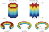 |
Figure 1 Identification of vertices of prisms (a) PR6 and (b) |

Solutions for this problem have been obtained for GML surfaces and bodies with m = 2, 3, 4, 5, 6 [1–6] and revealed connections with the field of knots and links, depending on the number of twists of the original cylinder or prism with m-symmetrical cross section, given by the superscript n in  . The method of study was the full cutting of
  surfaces and bodies with a moving knife in 3D. More general solutions were obtained when the cross section of the
 surface or body is a Gielis curve, describing the boundary of the cross section as well as the disk [4–7]. Gielis curves can transform the cross section of the
  from a circle to a regular polygon and vice versa, and to many other concave or convex curves. Hence using regular polygons allows for generalizing results to other convex figures.
Instead of a moving knife and fixed  , an equivalent approach is a fixed knife and a moving
  surface or body. Furthermore, using a fixed knife it is shown that the solution for the general problem of cutting regular
  surfaces and bodies can be obtained by studying the problem of cutting regular m-polygons in the plane, with di knives, where i is the ordinal number of the divisor and di is the divisor of m.
For example, considering VV cuts, a cut with a single knife d1 is made from vertex V to any other vertex dividing the polygon into two distinct parts. This can be repeated from vertex V1 to Vj, from V2 to Vj+1, etc., giving m possible cuts. A di knife with i = m on the other hand is a knife with m blades, achieving the same result as for d1 but in one cut.
The focus is on  bodies since the cutting problem will lead to separate sectors in the cross sections, and to separate bodies in one or more resulting GML’s. This problem has both a geometrical and a topological solution. In the former case, the number and the precise shape of the resulting bodies is counted, while in the topological case, only the number of sides and vertices of the resulting bodies is counted. For example, when the resulting shape is a quadrilateral, in the topological solution all quadrilaterals are treated as one solution, whereas in the geometrical solution the precise shape of the quadrilateral is important, e.g. a square. The topological solution is a subset of the geometrical solution.
The geometrical solution
Defining  as the number of ways of cutting an m-gon for a given divisor of m, whereby the superscript details whether this cut is a VV, VS or SS cut, giving
  ,
,  , respectively, then the total number of way of cutting with di = 1, …, m knives with i = 1, …, m blades is the sum of all possible cuts multiplied by the number of divisors.
The solution can be expressed as a recurrence relation in number of side-to-side cuts. Defining Nm as the number of ways of cutting an m-gon for a divisor equal to one, and  as the number of SS cuts for m and
  for the number of SS cuts for the polygon with (m − 2) symmetry, then for the geometrical solution the number of different ways of cutting an m-polygon with a dm knife is:
 (1a)
(1a)
 (1b)
(1b)
The total number is then the number of different ways in (1a) and (1b) multiplied by the number of divisors. In regular polygons the cuts  ,
,  have to be made from Vi → Vi+1, from Vi → Si+1, or from Si → Si+1 respectively. Vi → Vi, Vi → Si, or Si → Si do not divide the regular m-polygons into two distinct parts. As a corollary, in a convex polygon or a circle with equally spaced points however, such cuts are possible and the total number of cuts then has to be augmented by m:
 (2a)
(2a)
 (2b)
(2b)
The topological solution
The topological solution is given by the following general formula:
-
If m = 2k + 1 and has N nontrivial divisors d2, d3 … dN+1 and d1 ≡ 1, dN + 2 ≡ dm ≡ m, then the number of all possible variants of cutting of
 bodies is
![Mathematical equation: $$ {\mathrm{\Xi }}_m^{\mathrm{top}}=8k+1+3{Nk}+\sum_{i=2}^{N+1}\left[\frac{k}{{d}_i}\right]+2{N}. $$](/articles/fopen/full_html/2020/01/fopen200013/fopen200013-eq23.gif) (3a)
(3a)
-
If m = 2k and has N nontrivial divisors d2, d3 … dN+1 and d1 ≡ 1, dN + 2 ≡ dm ≡ m, then the number of all possible variants of cutting of
 bodies is
![Mathematical equation: $$ {\mathrm{\Xi }}_m^{\mathrm{top}}=8k-5+3{Nk}+\sum_{i=2}^{N+1}\left[\frac{k-1}{{d}_i}\right]-N. $$](/articles/fopen/full_html/2020/01/fopen200013/fopen200013-eq25.gif) (3b)
(3b)
The general formula can be expressed in the variables k and N, whereby m = 2k for even or m = 2k + 1 for odd numbers. di is the ith (i = 2, 3, … N + 1) non-trivial divisor of the number m, so N equals the number of divisors of m − 2 (excluding the trivial divisors dN+2 ≡ dm ≡ m, and d1 ≡ 1).  is the total number of divisors (including the trivial divisors m and 1) and square brackets […] indicate the integer part of the fraction. Also in this case the remark on convex polygons and circles is valid: the number of possible cuts has to be increased by m.
The occurrence of Möbius phenomena
The Möbius phenomenon, which led to the discovery of non-orientable surfaces for classical ribbons or strips, also occurs in GML surfaces and bodies. Möbius phenomena result in only one body or surface after full process of cutting when (a) m = even and (b) the knife passes through the centre of the cross section of GML bodies. The knives used in making VV, VS or SS cuts are chordal knives, dividing the m-polygon into two distinct parts and cutting the boundary of the m-polygon in exactly two points.
When using radial knives, which start from the centre of the polygon and cut the boundary of the m-polygon in exactly one point, it turns out that Möbius phenomena can occur both for m even and odd.
Generalizations and interrelations
This paper is organized in the traditional Greek geometrical way, with Propositio, Expositio, Determinatio, Constructio, Demonstratio and Conclusio. In the Expositio and Determinatio sections the focus is on paths towards generalizations and links to various well-studied problems in mathematics.
Generalizations include the circle or convex polygons, whereby Vi → Vi+1, Vi → Si, or Si → Si cuts are possible. Furthermore, it is by no means necessary to use straight (chordal or radial) knives as long as the knife-curve is wholly contained within the original domain. The precise shape of the knife can be the solution to some optimization problem. One generalization is cutting of concave polygons, whereby the knife is part of a “more-concave” polygon.
In cutting the polygon or convex shape, the resulting domains can be separated. However, the process of the knives is completely equivalent to connecting vertices and sides via drawing diagonals or connecting equally spaced points on a circle. Hence the problem of using m-knives to cut regular m-gons has a direct relation to other well studied problems in geometry, such as:
-
The problem of dividing m-polygons with non-crossing diagonals.
-
Number of separate parts in a circle when connecting all equally distributed points on a circle with straight lines.
The former problem was studied first by Euler and later by Segner, Lamé and Catalan. The solution of the problem is combinatorial and the results are the Catalan numbers. The combination of geometric and combinatorial problems (linked directly to permutations or identification of corresponding vertices (Fig. 1) in the problem of cutting GML) is very fruitful. Solutions to the second and related problems are other series of integer numbers, many of which are found in the Online Encyclopedia of Integer Sequences (OEIS). There are other relationships and many applications in physics and biology, and it opens a way forward to bridge topology and geometry within maths on the one hand, and mathematics and the natural sciences on the other.
Expositio
GML surfaces and bodies
 are torus-like surfaces or bodies, whereby the cross sections of the
  bodies are closed planar curves with symmetry m, and which are constructed by identifying opposite sides of a cylinder or prisms (Fig. 1) [1–4]. The planar curves with symmetry m can be regular polygons or any closed plane curve, including circles. GML surfaces are generated when only the curve itself, as boundary of a region is considered (Fig. 1 for
  , or bodies when also the disk enclosed by the curve is considered. For the classical cylinder or Möbius band, the cross section is a line, swept along a path forming a ribbon and twisted an even or odd number of times respectively. Whereas the lower index m determines the symmetry of the cross section, the upper index n describes the number of twists. GML surfaces or bodies can either be closed (Fig. 1) or not (Fig. 2). In the latter case they can be either sections of closed GML surfaces or bodies, or complete. They are called Generalized Rotating and Twisting surfaces and bodies GRT.
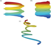 |
Figure 2 Examples of the GTR bodies which have different basic lines, radial cross-sections and numbers of twistings. |
Analytic definition of GML surfaces and bodies
Generalized Möbius-Listing Bodies  are defined by the analytic representation:
 (4)or, alternatively,
 (5)where p(τ, ψ) and q(τ, ψ) are given functions which can define surfaces of the radial cross section of bodies (Fig. 3), with:
-
a planar curve or disc as basic cross section (this can be a very general section, esp. Gielis curves or discs), which
-
can be swept around a closed or open path along a basic line (e.g., surfaces of revolution, or Monge surfaces), and which
-
can be given twists and turns as desired.
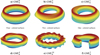 |
Figure 3
|

Permutations and colours
Each Generalized Möbius Listing’s body  can be considered as a geometric representation of the element of the permutation group [8], in particular:
 (6)
(6)
The sub-indices change from 1 to m − 1 cyclically and the sides are identified by the definition of  body. So it may be written as follows:
 (7)
(7)
The first row shows the identifications of the original prism and the second row the identifications after rotation and identification according to definition of  . These are elements of a special subgroup of the group of permutations, in which the number of elements of this subgroup equals m. The first row is always the usual sequence of numbers from 1 to m, and the second row may start from any number from 1 to m and then, given the cyclicity of the representation of numbers, their sequence is not changed.
Each element, except the neutral element, has a certain number of cycles, and geometrically, this directly relates to how many different colors can be painted on the surface of a given body, without lifting the brush and not passing the ribs. For example for m = 4 (see Fig. 3).
Corollary. Each  body has a j-colored surface where j =gcd (m,κ) and n = ωm + κ except when κ = 0, in this case we have an m-colored
  body [8].
From the original motivation to the general problem
The original motivation to study  is rooted in the study of boundary value problems and the geometrical description of natural shapes and phenomena [4]. The current study was initiated by the question what happens if the GML surfaces and bodies are cut along a certain line or surface, inspired by the cutting of the original Möbius band [2, 3]. For example, the result of cutting (d), (e) and (f) in Figure 3 along lines containing one vertex, will be very different.
Thus far, the classification of cutting of  surfaces and bodies was achieved for classic Möbius bands [3], and for
  with m = 2, 3, 4, 5 and 6 [4–6]. A full classification was achieved for cutting of classic Möbius bands with any k number of knives [3]. These classifications revealed a close link between the cutting of GML bodies and surfaces, the study of knots and links, and with the colouring of surfaces (Fig. 3). This can lead to intricate links of various separated GML surfaces and bodies (Fig. 4). In this case the cutting leads to ribbons, but if the
  Architon is a body the various structures will have different cross-sections.
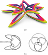 |
Figure 4 (a) |

The challenge remains to classify the cutting of general GML bodies when the cross section of the GML body is a regular m-polygon, for any value of m. This problem can be studied from several points of view, and it will be shown in particular that cutting planar regular m-polygons with a certain number of knives is an equivalent problem.
Demonstrations will be given for cutting with one knife or with m knives. Other ways of cutting, based on the divisors of m, are investigated, and the equivalence of cutting of  , the cutting of regular m-polygons, or in general Gielis curves and rotational symmetries of the circle with inscribed m-polygons will be considered, and the relevant connections to other fields of mathematics will be outlined. Using m-polygons does not limit the generality of our results. More details are provided in “Gielis curves, surfaces and transformations”, and “
Determinatio
” section.
, the cutting of regular m-polygons, or in general Gielis curves and rotational symmetries of the circle with inscribed m-polygons will be considered, and the relevant connections to other fields of mathematics will be outlined. Using m-polygons does not limit the generality of our results. More details are provided in “Gielis curves, surfaces and transformations”, and “
Determinatio
” section.
Gielis curves, surfaces and transformations
Gielis curves and transformations
The theory of GML surfaces and bodies was greatly enriched when it was merged with Gielis curves [7, 9–11], a generalization of Lamé curves or superellipses (A ≠ B) or supercircles (A = B) for any symmetry, defined as:
![Mathematical equation: $$ \varrho \left(\vartheta;A,B,{n}_1,{n}_2,{n}_3\right)=\frac{1}{\sqrt[{n}_1]{{\left|\frac{1}{A}\mathrm{cos}\left(\frac{m}{4}\vartheta \right)\right|}^{{n}_2}\pm {\left|\frac{1}{B}\mathrm{sin}\left(\frac{m}{4}\vartheta \right)\right|}^{{n}_3}}}. $$](/articles/fopen/full_html/2020/01/fopen200013/fopen200013-eq46.gif) (8)
(8)
The parameter m defines the symmetry and is thus related to the lower index of  The exponents n1,2,3 are not related to the upper index n of
  . Equation (8) can also be considered as a generic and geometric transformation on all planar functions, unifying a wide range of natural and abstract shapes [7]. Here we restrict the transformation on a constant function or circle, with A = B. Gielis curves (1) can serve both as cross section and as basic line around which the cross section is swept giving rise to GML bodies (Figs. 3 and 4). They can define:
-
Boundaries and disks, using the zones enclosed by the curves, technically using ϱ(ϑ) ≤ whereby the = sign defines the boundary.
-
Regular polygons with symmetry m are defined:
![Mathematical equation: $$ \varrho \left(\vartheta \right)=\underset{{n}_{1\to \infty }}{\mathrm{lim}}\left[\frac{1}{\sqrt[{n}_1]{{\left|\mathrm{cos}\left(\frac{m}{4}\vartheta \right)\right|}^{{2(1-n}_1{\mathrm{log}}_2\mathrm{cos}\frac{\pi }{m})}+{\left|\mathrm{sin}\left(\frac{m}{4}\vartheta \right)\right|}^{2\left(1-{n}_1{\mathrm{log}}_2\mathrm{cos}\frac{\pi }{m}\right)}}}\right]\enspace $$](/articles/fopen/full_html/2020/01/fopen200013/fopen200013-eq49.gif) (9)
(9)
-
Regular Gielis polygons sensu Matsuura [12] are generated for
 . A
. A  polygon is a very good approximation of a regular pentagon with m = 5, n2,3 = p = 1 and q = p(m/4)2. The difference between regular polygons defined in this way is less than 1% for m ≥ 5 and less than 0.5% for m ≥ 11.
 -
Self-intersecting polygons (m-polygrams) for m a rational number, are known as Rational Gielis Curves (RGC) [13]; for example for
 , a pentagram-like figure is generated. To complete the figure with 5 vertices, 2 rotations are needed, corresponding to the numerator and denominator of m respectively. In general, m can be rational (m = p/q with p, q relative prime), or irrational [7].
Furthermore, it is a continuous transformation, whereby any shape can be transformed into a circle, and then into any other shape [11]. The transformation is equal to 1, yielding the circle, for either m = 0 or limm→∞ The former is a zero-gon (or zero-angle), a figure without corners or vertices, while the latter is the classic notion of a circle as the limiting case of a polygon with an infinite number of sides. But the value is also equal to 1, and thus a circle, for n2 = n3 = 2, for any integer value of m (given A = B = 1). So if a pentagon is transformed into a circle, this can be done by changing the values of n2 = n3 for the pentagon to n2 = n3 = 2 (in a discrete or continuous way). However, even if this is a circle, it is also a pentagon, with the original equi-spacing of the five points on the circle still imprinted. The polygons can be transformed into circles, where the equidistant points are the roots of unity.
Pythagorean compact
Gielis curves are generalizations of Lamé curves using polar coordinates, and for n1,2,3 = n and n1,2,3 = 2 (given A = B, m = 4), we have Lamé curves and the classic Euclidean circle, respectively. Hence, these transformations have been named Pythagorean-compact. As all shapes are described in one Pythagorean compact equation, all shapes are equally simple, differing in a few numbers at most. Within the same Pythagorean structure, the arguments of the cosine and sine functions (in the original form  ) may be arbitrary functions f(ϑ), allowing for extremely compact form descriptions [14].
Moreover, all shapes can be continuously (or discontinuously if one chooses discrete steps) transformed into any other Gielis curve. The Lorentz transformation of Special Relativity Theory is one special case [10, 11]. There are deep connections to various other parts of mathematics, including Riemann surfaces, approximation theory and number theory. For the natural sciences, the main consequence is that the Gielis Formula allows for a uniform description of a wide variety of natural shapes, and their development [11].
Gielis surfaces and bodies
The two dimensional case can be generalized to [11]:
![Mathematical equation: $$ r\left(\vartheta,\phi \right)=\frac{1}{\sqrt[{n}_1]{{\left|\frac{\mathrm{sin}\left(\frac{{m}_1\vartheta }{4}\right)\mathrm{cos}\left(\frac{{m}_2\phi }{4}\right)}{a}\right|}^{{n}_2}+{\left|\frac{\mathrm{sin}\left(\frac{{m}_1\vartheta }{4}\right)\mathrm{sin}\left(\frac{{m}_2\phi }{4}\right)}{b}\right|}^{{n}_3}+{\left|\frac{\mathrm{cos}\left(\frac{{m}_1\vartheta }{4}\right)}{c}\right|}^{{n}_4}}}{.\alpha }\left(\vartheta,\phi \right). $$](/articles/fopen/full_html/2020/01/fopen200013/fopen200013-eq54.gif) (10)
(10)
As transformations of functions, with α(ϑ, φ) = 1 the unit sphere, Gielis transformations can be generalized immediately to any dimension [9]. Another way of defining 3D shapes is parametrically using two Gielis curves ρ1(ϑ), ρ2 (φ):
 (11)with a unit sphere for ρ1 (ϑ) = ρ2 (φ) = 1.
In this way a 3D Gielis surface or body can be defined on the basis of two perpendicular Gielis curves ϱ1(ϑ), ϱ2(φ). There are a variety of ways of defining surfaces and bodies, with Figure 4 as one example. In Figure 5 other examples are shown, showing both the equivalence of GML and special topological figures.
-
 body with one full rotation (circle as basis line).
 -
 with cross-section a circle or zero-angle, and basic line a ½ angle, (m = p/q = 1/2).
 -
 with basic line a one-angle or monogon (m = 1), no twists.
 |
Figure 5 (a) GML4 surface. (b) Torus with a Gielis curve with m = 1/2 as path. (c) A torus with path m = 1, giving rise to a Klein bottle. |
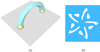 |
Figure 6 (a) Upper half of GML meeting Flatland, with the green and the red dot connected via a rib. (b) Architon (Fig. 4) moving through a cone. |
Figure 5c is a monogon with basic line parameters m = 1, A = B and all exponents n in equation (8) equal to 1. When this 2D curve is transformed into a torus, it becomes the Klein bottle. It is remarked that in all cases the cross sections are constant, but they can also be scaled or morphed when swept along the basic line, resulting for example in vortices. In 3D a sphere can be transformed into a torus in a purely geometrical way, since the 3D parametric version is based on two perpendicular sections [11].
When transforming a sphere into a torus one of the cross sectional circles, increases in size. In Figure 5b, a torus transforms into the half-angle shape ( ), which leads to a torus with two holes. Actually, by having value of m in the Gielis formula as 1/p with p an integer, tori with any number of holes equal to p can be generated. The number of holes corresponds to the genus of a surface. One example is the half-angle torus in Figure 5b, which has two holes, or genus 2. In Figures 1, 3, and 7, the basic line of the GML surfaces and bodies is a circle, but this can be any knot-like structure or RGC, such as a pentagram.
 |
Figure 7 (a) Pentagonal GML body. (b) One of the resulting structures. |
The equivalence of cutting GML bodies and m-polygons
GML meets Flatland
At the end of the 19th century E. Abbott wrote Flatland, a story of dimensions [15]. The goal was to show how people could think about four-dimensional space, by considering Flatland and its inhabitants. When a sphere moves through Flatland, the inhabitants will initially see a circle that starts as a point, increases in size, until the maximum size is reached. Then it will decrease until it disappears again, leaving the Flatlanders in shock and awe. Only when one of the Flatlanders travels into 3D space, (s)he realizes what truly happened, but ultimately finds  self in great difficulty trying to explain this to fellow inhabitants of Flatland.
We can take the same approach. A GML body or surface is a 3D torus-like surface or body, with certain symmetry. Figure 6a displays part of a GML body with square symmetry. The GML surface or body crosses Flatland (Fig. 6a) and the yellow zones are those observed by inhabitants of Flatland. However, they cannot discriminate between the different orientations of the square, resulting from a twist in 3D and indicated by red and green dots. Figure 6b displays a snapshot of Architon (Fig. 4) moving through Coneland. To a Conelander various unconnected and mysterious shapes are observed. Undoubtedly to a Flatlander or Conelander, mysterious things happens if such structures move through their territories. What the Flatlanders or Conelanders will notice – a boundary or a disk – depends on whether GML is a surface or a body. In advanced societies like Flatland and Coneland, its physicists may develop methods to find out whether the shapes are boundaries or disks.
Figure 7a displays part of a complete GML body with pentagonal cross-section, cut from side to side, cutting the cross sections into two distinct parts. If the cutting process is continued along the whole twisted GML body until the knife arrives at the very same position as the initial one, eventually four different bodies will result, one triangular one in light blue and one quadrangular one in brown, and two pentagonal ones, in yellow and grey. Each body or surface will be twisted in a certain way, fully predictably.
Figure 7b displays only one of these shapes, but in fact, after cutting, all four structures are intertwined into one complex shape. An inhabitant of Flatland will only see the overall pentagonal cross section as in Figure 7a, which is cut from side Si to Si+2 with five knives, showing the equivalence of cutting GML bodies and regular polygons. Alternatively (s)he may see a number of disconnected shapes, ten triangular or quadrangular shapes (either blue as in Fig. 7b or brown) and six pentagonal shapes (in grey and yellow).
Cutting bamboo poles
When cutting GML with one (or more) knives, one can consider the knife moving along a rib on the GML body as in Figure 6a. In this case the knife corresponds to one of the diagonals of the cross sections, keeping a constant orientation relative to the cross section, e.g. along one rib of the GML body. Alternatively one can fix the knife and move the body through the knife. A real life example of cutting with various knives is found in hand tools or in machines used for splitting bamboo culms (Figs. 8a and 8b). The knives can be adjusted to split the bamboo in any number of pieces. These culms are hollow, but one can easily imagine the same procedure for full prisms. In case the prisms are twisted and closed in a GML fashion, the results with one knife or more knives will be the same.
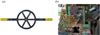 |
Figure 8 Knives and machines for splitting bamboo [16]. (a) Hand-operated tool moved to split a fixed culm. (b) Bamboo splitting machine with fixed knife and moving culm. |
Cutting regular m-polygons with one knife
Having established the equivalence of cutting GML and polygons with a moving or fixed knife, now consider the regular m-polygon with rotational symmetry m ∈ ℕ, i.e. a regular polygon with m vertices and m sides connecting the vertices. There are three ways of cutting a regular m-polygon. A cut, which divides the structure into two distinct zones, can be made from:
-
vertex to vertex VV, with notation VVi,j, a cut from vertex i to vertex j,
-
vertex to side VS, with notation VSi,j, a cut from vertex i to side j,
-
side to side SS, with notation SSi,j, a cut from side i to side j.
In the case of VV the first V is labelled as V1 so that a cut from the first vertex to the third vertex, in clockwise direction is called VV1,3, which is for example the diagonal of a square (Fig. 9a).1 The first index i of VVi,j, VSi,j and, SSi,j refers to the first letter, and the second index j refers to the second letter (V or S). In the case of vertices and sides, the labelling both starts at 1, so at V1 and S1. Then VS1,2 defines a cut from V1 to S2, which lies inbetween V2 and V3 (Fig. 9b). If a cut passes through the centre of the polygon, it is denoted as subscript C (Figs. 9a and 9c), although this notation may be dropped in obvious cases as in Figure 9a. In Appendix all possibilities are shown for m = 6, …, 10.
 |
Figure 9 Ways of cutting of a square, left to right: (a) VV1,3,C (b) VS1,2 (c) SS1,3,C (d) SS1,2. |
Notes
-
A cut is similar to drawing a straight line connecting vertices to vertices or sides, and sides to sides. Straight vertex-to-vertex lines are also known as diagonals.
-
A single cut divides the regular m-polygon into two distinct parts, i.e. the knife is part of a line, which has exactly two points in common with the boundary of the polygon. Such knife is called a chordal knife, analogous to the chord cutting a circle, giving rise to definition of sines and cosine. In Figure 8a the bamboo knife can be considered as three chordal knives through the centre.
-
Cuts, which are symmetrical with respect to clockwise or counter clockwise rotations are counted as one. If clockwise rotation is indicated as + and counter clockwise as −, then e.g. VS1,−2 = VS1,2
-
VVi,i+1 or VVi,i−1 cuts are excluded as they coincide with a side and do no divide the polygon into two distinct parts. When cutting convex polygons with curved sides [4], or circles with equally spaced points VVi,i+1 or VVi,i−1 are possible.
The number of ways the m-polygon can be cut with one knife is equivalent to drawing one line. The total number of cuts is 3k − 2 for even numbers m = 2k, and 3k − 1 for odd numbers m = 2k + 1 (Tab. 1). For increasing m this leads to the following:
-
From m odd to m + 1 (even) the number of possible cuts increases with 2, namely VV1,(m−2) and SS1,(m−2). For example, in m = 6 the new possibilities are VV1,4 and SS1,4, compared to m = 5.
-
From m even to m + 1 (odd) the number of possible cuts increases with 1, namely VS1,(m−2). For example, for m = 5 the new possible cut is VS1,3 compared to m = 4.
Possible cuts for m-polygons m = 3, 4, …, 7 and the general case.
This is equivalent to an increase with three possibilities going from m to m + 2. From m odd to m + 2 (odd), or from m even to m + 2 (even), the number of possible new cuts increases with 3 in both cases. The number of possible cuts in Table 1, right column, is the sequence 2, 4, 5, 7, 8, 10, 11, 13,… and this sequence (from odd to even plus 2 and from even to odd plus 1) will be continued for any increasing value of m. In the OEIS database of integer sequences, this sequence of numbers is: numbers not divisible by 3.
Divisors and different ways of cutting
The cuts described above (Fig. 9 and Tab. 1) are made with precisely one knife corresponding to the smallest divisor of m, namely 1. The number of cuts with 1 knife is equivalent to divisor d1. The results of cutting GML with regular polygons as cross-section or cutting regular polygons, aligns with the number of divisors of m.
The number of divisors d of m ≥ 2. The number of divisors is 2 if and only if m is a prime number and the divisors are then d1 and dm. The smallest divisor d1 is always 1 and the largest divisor dm is always equal to m. For all values of m, the divisors are designated d1, d2, …, dm.
Cutting with m knives is equivalent to the largest divisor dm. Using d1 or one knife the cut started either in V1 for VV and VS cuts, and from S1 for SS cuts. For divisor dm or m knives, cuts start in all m vertices and on all m sides. The cuts are symmetrical to the case d1 of one knife.
The cuts are based on repetition of d1 cuts, by rotation, for example for hexagons and VV and VS cuts:
-
VV cuts based on VV1,3: VV1,3, VV2,4, VV3,5, VV4,6, VV5,1 and VV6,2
-
VV cuts based on VV1,4: VV1,4, VV2,5, VV3,6, VV4,1, VV5,2 and VV6,3
-
VS cuts based on VS1,2: VS1,2, VS2,3, VS3,4, VS4,5, VS5,6 and VS6,1.
-
VS cuts based on VS1,3: VS1,2, VS2,4, VS3,5, VS4,6, VS5,1 and VS6,2.
VV and VS cuts result in four different figures for both d1 and dm = 6 (Fig. 10a), but with a one-to-one inheritance from d1 to d6 (or vice versa) i.e. the same total number of figures, namely 4. Additional possibilities will be created however, when m side-to-side cuts are considered for dm.
-
SS cuts based on SS1,4: if the cut is made from the middle of S1 to the middle of S4, the cuts cross the centre of the hexagon (Fig. 10a, column SS1,4). In this particular case m is even, and the line contains the centre of symmetry.
-
For SS cuts based on SS1,2 or SS1,3 the result depends on whether the cuts are made from
-
the middle of S1 to the middle of S2 or to the middle of S3;
-
side to side such that the cutting line is shorter or longer than the cut from middle to middle.
-
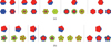 |
Figure 10 (a) Cutting a hexagon with 1 (d1 upper row) or 6 knives (d6 lower row). (b) Cutting a pentagon with 1 (d1 upper row) or 5 knives (d5 lower row). |
This is shown in Figure 10a, columns SS1,2 and SS1,3. In total, five additional different ways of cutting result for dm compared to d1. For the hexagon, for d1 the total is 7, for dm = 6, it is 12.
The results for cutting a pentagon with 1 knife (d1 = 1) and 5 knives (dm = 5) are shown in Figure 10b. For d1 there are five possibilities. The additional VS1,3 for dm = 5 compared to a square, is generated when the cut is made through the centre of the pentagon. For dm = 5 the total number is 12, as for dm = 6 in a hexagon. For SS1,3 there are four additional ways of cutting, compared to d1 that fall into two categories.
-
First, as in the case of the hexagon, the cut SS1,3 can be made parallel to the side of the pentagon, again, from middle of S1 to exact middle of S3, or shorter, or longer, giving four extra possibilities as for the hexagon.
-
Second, the cut SS1,2 gives rise to an additional two possibilities, depending on the cut made. From left of middle of S1 to right of middle of S2 or from right of middle of S1 to left of middle of S2.
Going from a pentagon to a heptagon (Fig. 11), the total number of ways of cutting for dm = 7 is 17. Two extra vertices and two extra sides generate additionally VS1,4 and SS1,4. The former generates one extra possibility of cutting (Fig. 11 column VS1,4) like VS1,3 in the pentagon, while the latter generates 4 extra possibilities (Fig. 11 column SS1,4), like SS1,3 in the pentagon, compared to d1. SS1,3 and SS1,2 generate three possibilities each, again dependent on where the cut is made (Fig. 11 columns SS1,3 and SS1,2). This pattern will always continue going from m to m + 2 for m odd. A similar reasoning leads to same conclusion for m even.
 |
Figure 11 Cutting a heptagon with 1 or 7 knives. |
For dm the number of ways of cutting increases according the following rule: When m increases from an even number m = 2k to the next odd number m = 2k + 1, the number of possible cuttings increases by 5. When m increases to the next even number m = 2k + 2 the number of possibilities does not change.
For m = 3, 4, 5, 6, 7,…. the number of possible cuts dm is the monotonic sequence 7, 7, 12, 12, 17, 17, 22, 22,… or taken two by to 14, 24, 34, 44… In general, for couples m = 2k − 1 and m = 2k this gives (k − 1) ∙ 10 + 4.
Geometry versus topology
The main difference between dm and d1 is that in d1 certain cuts are not differentiated. For example in SS1,4 in Figure 11, the line connecting sides 1 and 4, can lie anywhere on both sides. For dm however it is important where exactly sides 1 and 4 are cut. In Figure 9 column SS1,4 the cut can go either through or not through the centre of the regular hexagon. When it does not go through the centre, various objects are generated, indicated by different colours.
This is the difference between the geometrical and topological identification of the solution, indicated in Propositio. In SS1,4 in Figure 11, any cut with one knife (upper row) will generate two pieces, one with five vertices, one with six vertices (the topological condition). If the cuts with one knife need to generate shapes, which are one to one congruent (the geometrical condition) to the dm case, also the upper row will have five different variants.
In Table 2, the number of ways of cutting a regular polygons for smallest and largest divisor is given, and the total ways of cutting in the topological sense, the sum d1 + dm.
-
From an even number m2n to the next even number m2n+2: d1 + dm = +8.
-
From an odd number m2n+1 to the next odd number m2n+3: d1 + dm = +8.
Number of cuts for smallest and largest divisors for m-polygons.
The general rule is: The number of possibilities of cutting a regular m-polygon with one or (m) knives (d1 + dm) is the number of possibilities of cutting a (m-2)-polygon increased by 8. As a consequence of the number 8 increase, the sequence of numbers 9, 11, 17, 19, 25, 27, 33, 35, … is (1,3) modulo 8, i.e. the numbers of d1 + dm are divisible by 8 with remainder 1 or 3. In Table 2 the total number of possible cuttings for smallest and largest divisor of an m-polygon is given up to m = 10. The value of d1 + dm for odd m is 1 modulo 8 and the value of d1 + dm for even m is 3 modulo 8.
The total number of possible cuttings for smallest and largest divisor of an m-polygon is always an odd number. It is 4m − 3 (or 1 mod 8) for odd values of m and 4m − 5 (or 3 mod 8) for even values of m. The total number of ways of cutting an m-polygon for m = prime is (d1 + dm) = 4m − 3 or 1 mod 8.
So we have the following:
Lemma 1
In the topological sense, the cutting with one knife (d1) gives the minimum number of cuts, while cutting with m knives (dm) gives the maximum number of cutting variants. In the geometrical sense, the minimum number of cutting variants (with a d1-knife) equals the maximum number of cuts (dm-knife).
GML versus polygon cutting with 1 or m knives
The original study is a moving knife cutting 3D-Generalized Mobius Listing bodies (Fig. 6) and continuing until the knife returns to the initial position (i.e. a complete cut). In Table 3 the cutting using a largest and smallest number of knives, related to smallest and largest divisors, is presented for GML cutting with moving knife. The condition n = km corresponds to full rotation and d m = 1, and the condition n = km + j(gcd(m,j) = 1 to dm = m.
GML cutting with moving knives.
Table 4 gives a summary. Comparison with Table 2 totals shows that the correspondence of GML cutting and regular polygons is indeed complete.
Comparative table for GML and polygon cutting.
Defining knives for all divisors
For d1 cuts are made starting from V1 or S1 . For dm this operation is repeated every 2π⁄m. For divisors other than d1 or dm, the operation has to be repeated less than every 2π⁄m. In Table 5 the rotations which have to be performed is indicated for m-polygons with more than two divisors for m = 4, 6, 8, 9 and 10. The denomination d3 = 4 indicates that for m = 8 having four divisors 1, 2, 4 and 8, the third divisor is 4. The denomination dm always refers to the highest divisor, in this case equal to dm = 8 for the octagon. The rotations are k·2π/m. The value of k depends on the other divisors. For example for m = 10, k = 5 for d2 = 2, k = 2 for d3 = 5, k = 1 for dm = 10 and k = 10 for d1. The results are shown in Figure 12 for m = 4.
 |
Figure 12 Ways of cutting for a square for all divisors d1 (upper row), d2 = 2 (lower row) and dm = 4 (central row). |
Traces of d-knives.
This then leads to the following analytic definition of di=1,…,m-knife: the di-knife is a construction, with m straight lines [8]:
 (12)
(12)
![Mathematical equation: $$ {y}_i=\mathrm{tan}\left(\alpha +\frac{2\pi }{m}i\right){x}_i+{\delta \left[\mathrm{cos}\left(\alpha +\frac{2\pi }{m}i\right)\enspace \right]}^{-1},\enspace {i}=0,\enspace 1,\enspace \dots,m-1;\enspace -\frac{\pi }{m}\le \alpha \le \frac{\pi }{m}. $$](/articles/fopen/full_html/2020/01/fopen200013/fopen200013-eq62.gif) (13)
(13)
The parameter α is a rotation parameter and δ is a dilation or zooming parameter. With these parameters all possible ways of cutting can be described. In Figure 12 middle row one can observe how the red square is dilated and rotated. Dilation can shrink the square to a point as in the VV1,3 and SS1,3 cut through the centre. This will be used in
Demonstratio
section “Rotations and scaling” since this is equivalent to projection. In evaluating other divisors, the value of i should be amended, according to Table 5. For example, in the octagon d3 = 4 the cut is repeated every 90°, or i = 2:  or 90°.
For d2 = 2 (equivalent to m = even) the number of possible ways of cutting in the topological sense is the number of possibilities for d1 + 1. In evaluating the number of divisors in relation to GML or regular polygon cuts, it is found that for VV and VS all divisors are equal for even m. For odd m the same goes for VV cuts, but for VS cuts one has to take into account whether or not the cut goes through the centre, at least in the topological sense. The number of ways of cutting VV or VS is in geometrical sense inherited one-to-one from VS or VV cutting for smallest and largest divisors, basically this number is constant for all VS, VV cuts for all divisors.
The challenge will be determining the regularity for SS cuts. In enumerating the total number of ways of cutting of m-polygons, we need to take into account the fact that we do not know a priori how many divisors m has (https://oeis.org/A000203).
The divisors of a number m may be numbered from minimum to maximum (min and max) leading to the following sequence:
 where:
-
dmin is the smallest divisor (always equal to 1) and,
-
dmax is the largest divisor (always equal to m).
A number has either even or odd number of divisors e.g. (1, 2, 3, 4, 6, 12) for 12 and (1, 3, 9) for 9. If the number of divisors is odd, the sequence has a central value (e.g. 3 in sequence for 9), but this may be used twice, so the sequence is (1, 3, 3, 9) as in (1, 2, 4, 4, 8, 16), so that all numbers have an even number of divisors.
The divisors can be grouped pairwise as:

-
For m = 9 the pairs are (1, 9); (3, 3).
-
For m = 12 the pairs are (1, 12); (2, 6); (3, 4).
-
For m = 16 the pairs are (1, 16); (2, 8); (4, 4).
The products of these pairs are always equal to m. When relating this to rotational symmetries C for m = 12, the pairs are (C1, C12); (C2, C6 ; (C3, C4) and these relate to the spacing of equidistant points on the circle, and the angles between them. For example, C2, C6 points are spaced 180° and 60° apart, respectively, corresponding to the rotation parameter for divisor 2 and 6.
Back to Flatland
The cutting of regular polygons is an equivalent method for demonstrating the general cutting of  , with a one-to-one correspondence of the cutting of regular polygons and the cross sections of
  bodies. As a consequence the problem may be reversed as follows:
Given the possibility of cutting planar regular m-polygons (as discussed in Section “ Expositio ”) obtained with a number of knives equal to d1, d2 …., dm , can the same result be obtained using only one knife?
The answer is affirmative, if the operation is carried out in 3D, via GML bodies with a specific number of twists.
But what does an inhabitant of Flatland observe when operations with 3D  bodies or surfaces are carried out, in other words, when
  bodies rotate through Flatland? Or, when
  bodies do not rotate but the knives are moving? Or when we position the fixed knife in Flatland with rotating
  bodies?
An inhabitant of Flatland may observe at some instance in time what looks like a pentagonal piece of paper lying on his/her desk, and may place one knife across the paper (VV, VS or SS direction). Next morning the Flatlander may wake up to see how the whole situation is still the same. However, it might also be that the “pentagonal piece of paper”, which is actually a planar section of a  , rotating through Flatland, is sliced into different zones (Figs. 7a and 10b); how many zones depends on the number of twists of the
  and the number of rotations through Flatland. The Flatlander may also use more knives. He or she does not have to do anything at all; one dimension higher a rotation of the
  may have occurred.
Performing this with a square, somewhere else in Flatland a second, identical operation has happened. If both Flatlanders come into contact with each other, they will find that the square is somehow turned 90° (Fig. 6a). In classic Euclidean geometry, one cannot distinguish between two squares rotated 90° or a multiple thereof. If the  bodies are twisted, experimental identification of differences may be performed on the ground. In one case the diagonal runs “North to South”, in the other one “East to West”.
Without knowing the GML structure and number of knives, a Flatlander is bamboozled by this spooky action at a distance. If the Flatlander tries to untangle the mystery, by repeating or experimentally using other knives and positions, this will result in fully predictable structures, and reproducible phenomena elsewhere in Flatland, for example diagonals in the two squares in the same or different directions. The diagonal also has direction, like a spin, and the one influences the other. This is reminiscent of quantum entanglement, now via GML bodies and cutting.
Figure 6a shows a GML touching Flatland as a plane. Only half of the GML is shown, and the second half is beneath Flatland. But when the plane is folded, the complete GML body or surface can become a generalized cylinder (Fig. 13). This cylinder can be a complete GML or it can be part of the GML. In the latter case the GML can be closed either in 3D by a completed GML, not shown in the figure and not touching the Brane, or by direct connections on one side of plane or brane (think streamlines, an electronic circuit or graph). In addition, the width of the GML need not be constant, so it can be a generalised cone, a generalized hyperboloid, twisted beams or wormholes instead of a generalized cylinder. The brane in Figure 13b is a fold of the planar surface in Figure 6a, and the grey surface of Figure 6a or the grey surfaces of Figures 13a and 13b themselves can be folded topologically into a torus. The GML body then connects the surface of the torus like a fistula within the torus (Fig. 13), or a surface or body of genus 2 results, whereby the upper half of the GML in Figure 6a is a handle.
 |
Figure 13 Partial or complete GML bodies, with cross sections in Braneland. |
Actually, the cutting via divisors or via knives can also be considered as a process of projection, whereby a certain shape is projected onto a basic shape. The rotation and zoom parameters define the projection. In Figure 13 the upper yellow zone is projected onto the lower part of the brane, along the GML. In Figure 12 middle row for example a red square is projected on to a base square of fixed size (blue). This projection can be performed with a square for dmax = 4, with a line for dmin = 1 or with a rectangle for d2 = 2. One can observe from Figure 12 that this gives similar results as cutting with d knives and rotations. Projection may occur via a classic cone, a pyramid, a prism or via any projective device, for example with varying width in the GML, even when the width becomes small as in a vortex, or goes to zero.
Chordal and radial knives
In previous publications it was shown how in some cases the process of cutting leads to the Möbius phenomenon. Based on the current method of cutting, the Möbius phenomenon only occurs for m-polygons under two conditions: (1) m is even, and (2) the cut is made through the centre. It does not occur in any case of m odd, since the first and foremost condition is a geometrical one: the shapes have to be congruent after rotation to be able to form a single body! If m is odd there is no case in which cutting leads to a single body for the pentagon.
Thus far only cuts were from perimeter to perimeter (including no, one or two vertices), cutting the planar polygons into two different parts. These knives are chordal knives, since it relates to a chord in the classical sense. However, one can consider also shorter knives. A knife starting in the centre and passing through one vertex or side is called a radial knife. The notion of m-knives, chordal or radial knives can be viewed in a broader perspective. In this sense chords and radii are intervals of a line and half-line respectively, falling wholly within the m-polygon or circle and having at least one point in common or more for self-intersecting shapes (Fig. 14). It is noted that curves can be defined in this case as regular Gielis polygons sensu Matsuura [12]. The pentagon is a  ; the pentagram is
  and the circumscribing circle is G5,1,2.
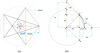 |
Figure 14 (a) Radial (red, dotted + solid) and chordal (yellow) knives. (b) Classical trigonometric functions. |
In a circle, the length of the radius is half the length of the longest chordal knife (Fig. 14). The inspiration can be found in botany once more: when sawing wood, one can use radial or tangential cuts. The latter is a chordal cut. When this cut is from vertex to vertex, the chordal knife may also be called a diagonal knife.
A more refined definition is then:
-
dcc chordal knife, through the centre C (e.g. SC cut in odd m polygon),
-
 chordal knife, not through the centre,
 -
drc radial knife originating at the center,
-
 radial knife not through the centre.
The -knife is defined for completeness, but is a special case of a chordal knife with length shorter than the chordal one). A radial cut drc is also a half-line or ray.
Interestingly our knives, as part of lines and half-lines, can be considered in a very classical way: When cutting a polygon, e.g. a pentagon (Fig. 14), the circle circumscribing the m-polygon, has the vertices in common (as roots of unity). A chordal cut (the yellow line in Figure 14a is a VVi,i+2 cut; the dotted lines are VVi,i+1 cuts) then connects two points on the circle, and defines the associated trigonometric function sine (chord = 2.sine), which is maximal when the chordal cut is through the centre and minimal when cutting only one vertex. In this case the chord, when prolonged, is the tangent to a point on the circle. This chordal cut can be taken from any point to any other point on the circle, and the perpendicular can be drawn, which defines the cosine. Indeed, the cosine is defined by drawing the perpendicular to the chord through the centre (Fig. 14a red). This divides the chord into two equal pieces.
Prolonging the red perpendicular (the cosine) to both sides gives the diameter. The max value of the cosine in a unit circle with radius R = 1 is also the magnitude or length of the normal to the circle (radius of curvature). Hence tangent and curvature are defined in the same setting. Figure 14b shows the relation with other classical trigonometric functions. A radial knife has length 1, and is the sum of cosine OC and versine2 CD, or the sum of sine OG and coversine GH.
Using chordal or radial knives the results of cutting will be the same for GML surfaces and bodies, but the distinction will become very important when discussing the occurrence of the Möbius phenomenon. Chordal knives cut the boundary, but it is also possible to define knives defined by a Jordan curve completely contained inside the original boundary. In this way two zones are created. If the inner zone is then cut with chordal or radial knives, similar results are obtained. If in Figure 14 a knife is used corresponding to the thick pentagon inside, then the inner pentagon is separated from the rest of the original  body. When radial or chordal knives are used, the same way of cutting gives the smaller pentagram. This can be continued ad infinitum.3
Determinatio
In Expositio it was shown that the processes of cutting GML bodies or m-polygons are equivalent and related to the divisors and the number of knives. This equivalence will be used later for the demonstration and proof. In this Determinatio section, it is investigated how the process of cutting is related to the theory of knots and links, the distribution of points on the circle (roots of unity), the ways of cutting a polygon, graph theory, the theory of numbers and primes, combinatorial aspects, etc. In this way many viewpoints are combined from various areas (geometry and algebra), with a very broad applicability for the general results of cutting of GML surfaces and bodies.
One crucial point of this solution with d-knives (radial or chordal), is that this solves a problem concerning 3D shapes and bodies using 2D geometry. In Riemannian geometry for example, one can determine the sectional curvature of an n-dimensional manifold, by determining the curvatures of planar 2D-cross sections in the tangent spaces [17]. In the same way, the current method would allow to solve problems in n-D GML bodies and surfaces, by studying 2D sections and solutions.
GML bodies and relation to knots and links after cutting
The use of planar geometry and cutting aims at providing a proof/demonstration for the cutting of GML bodies and surfaces. At first it makes abstraction of the intrinsic complexity of the cutting process, namely the number of bodies that are generated, how they are twisted and how they are interconnected. Indeed for 3D GML surfaces and bodies, the shapes can be very complex, and a full classification has been achieved for m = 2, 3, 4, 5, 6. The case 2 refers to ribbons, but can also be 2-angular figures [1–6].
We recall some results from [5]. In Figure 15a the results are shown for cutting a  body, which is twisted 4ω times (e.g. a full rotation over 360°; compare Fig. 3, but ω can be 0 for untwisted prism). For example the SS1,2 (A) generates both a triangular and a pentagonal shape and depending on the initial value of ω, the shapes are twisted 3 and 5 times respectively. The complete structure consists of the two shapes interlinked (Link-2). This situation corresponds to cutting with 1 knife or d1 (note that the SS1,3 and SS1,3,C cut give the same result so that total number is four).
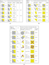 |
Figure 15 Cutting (a) |


The SS1,3,C cut of Figure 15b (BII) generates a single shape whereby the original shape is twisted 8 times (8ω + 8 for ω = 0, 1, 2, …). These situations correspond exactly to cutting squares with two knives or d2 = 2 in section “GML versus polygon cutting with 1 or m knives”, with five possibilities, one more compared to one knife. In Figure 15c the same shapes are generated as cutting with four knives or dm = 4 in Figure 12 central row. The essential aspect of cutting GML surfaces and bodies, and one of the original motivations is that the result of cutting leads to linked bodies with a certain link number (right columns). The surfaces or bodies may be knot like or display the Möbius phenomenon, with one shape and Link number 1, and this occurs in BII and D in both Figures 15b and 15c (for m even).
In Figure 16a, in the left column 8 ways of cutting are used, instead of the 5 ways in Figure 10. These 8 ways however, can be reduced to 5 since in this way of cutting the centre of the pentagon is not important:
-
All SS1,3 cuts (Ba, b, c) yield exactly the same results, namely four angular bodies and five angular bodies with the same link-2 number.
-
Both C II cuts (CIIa and CIIb), also yield the same result.
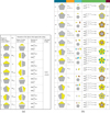 |
Figure 16 Cutting (a) |


Hence the number of ways reduces to 5 if we consider topological solution, taking into account only the number of vertices and sides.
In Figure 16b in the left column we have 12 ways of cutting with one knife, instead of 5. But here in all cuts except VV1,3 the position of the cut is important, depending on whether it is made above, through or below the centre of gravity of the pentagon:
-
SS1,2 has three possible ways of cutting (AI, AII, AIII).
-
SS1,3 has five possibilities (BI, BII, BIII, BIV and C).
-
VS1,3 has two possibilities (E and F).
This explains the difference between 5 ways of cutting for d1 and 12 ways for dm giving a total of 17.
Projecting and rotating shapes
The methodology used above refers to cutting or drawing lines, from side to side, vertex to vertex, vertex to side, either containing or not, the centre of the shape. The shapes can be considered as the result of projection. The transformations rotation and dilation or scaling, show how all these shapes fit together. Focus is on two basic shapes, the invariant one, and the projected one. In section “Defining knives for all divisors” the analytic presentations describing the knives (Eqs. (12) and (13)), have parameters α and δ, dealing with rotation and dilatation, respectively.
In Figure 12 onto a basic square, other shapes are projected (square, line or rectangle), related to divisors. For d1 a line is projected (upper row; imagine a line by a laser cut); for d2 = 2 a rectangle is projected (lower row; in case of VV1,3 or an SS cut through the centre the rectangle reduces to a line); for dm = 4 a square is projected (middle row). The line can be projected in any way, in any position. In Figure 15c right column, a grey rectangle is projected onto the yellow square. This rectangle can be narrowed and rotated. In Figure 15c (right column) a grey square is projected onto a yellow basic square (AI) and scaled (AI → AII → AIII), then a rotation AIII → BI, a scaling BI → BII, a rotation BI → C or a rotation BII → D. In Figure 17 this is shown as a projection along the ribs of a pyramidal cone (see also Fig. 12 central row).
 |
Figure 17 Projections along a pyramid. The solid blue lines are cutting lines. |
For the pentagon (Figs. 10 and 16) the same arguments can be made. In Figure 16b, onto a yellow base pentagon, a grey pentagon is projected (AI) and scaled (AI → AII → AIII → G → BIV). The grey pentagon is rotated 36° compared to the yellow pentagon. It can also have the same orientation as in BI and BII. Other instances are related to orientation.
This connects to the classical theory of conic sections, albeit that the cones can have a square cross section (a pyramid) or cross sections of any regular m-polygon, and this cone can then be moved through a fixed m-polygon. In the broader setting of  and Gielis curves there is no restriction to prisms. The base cross-section, can be swept along a central line, or diminish in size, as in a cone (Fig. 17), and need not to be constant.
Equidistant points on the circle
Since all Gielis curves, including self-intersecting curves, can be mapped onto the circle by a continuous Gielis transform, all vertices of an m-polygon can be mapped onto the circle. The vertices of a polygon are equispaced points on the circumscribing circle. The inner and outer vertices from a self-intersecting regular polygram, will become equi-spaced points on a circle, but they will be rotated relative to each other (Fig. 18 for m = 23). They can also be coinciding points. In this way, the same phenomena can be studied as points on a circle, using either algebraic approaches (groups and subgroups of the circle) or using geometric-algebraic approaches (Fourier, Chebyshev, complex numbers, etc.). All circles can be mapped onto one circle, or smaller and larger circles can be used (Fig. 18). The self-intersecting Gielis curves, giving rise to multivalued functions, are directly related to Riemann surfaces. Note that a VV1,2 cut is possible in the circle, whereas in regular m-gons such cut coincides with a side (it does not cut of a separate sector). VVi,i+1 cuts (e.g. V1 → V2) do divide the circle into two distinct parts.
 |
Figure 18 Connecting equally spaced points on a circle (the circle itself is not shown, only connections; when m is even, connections pass through the center). |
Shortest path and curvature
To go from one point to another point on the curve, if the curve is the only possible way to go, one best follows the curve itself, and this then is the shortest path. Assume a circle, a Lamé curve with exponent n = 2, and an inscribed square with n = 1 (Fig. 19a). Then the inscribed square, similar to the diagonals connecting four equally spaced points, or using all possible VVi,i+1 cuts, can be considered as the knives cutting the circle. The straight cuts are the shortest possible ways, using the isotropy of the Euclidean plane.
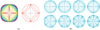 |
Figure 19 (a) Lamé curves for n = 2/3, 1 and 2. (b) Gielis curves for m = 1, 2, 5, 6. Each figure shows various curves for different exponents [18]. |
However, if one considers Lamé curves with 1 < n < 2 or n < 1, curves connecting the points result. They are curved lines, but using a broader definition of curvature, they are the shortest points to connect the two adjacent points on the circle.
From another viewpoint, the outer curve can have one geometry/curvature, while inside it can have another metric/measure/geometry/curvature, using another Lamé or Gielis curve. Now consider the three Lamé curves in Figure 19a as separate curves, and suppose that the red lines define a height function, e.g. they are elevated 1000 m above the plane.
Then the only way to travel along the circle or any of two other curves safely is to follow precisely that curve. If the circle and the inside square are considered, the circle as the outer curve and the inscribed square as the four knives, both at elevation of 1000 m, with deep down active volcanoes, tigers, lions and snakes, then it is possible to take different routes to travel from one point to the other, either via the square or along the circle. Connecting two of the four points is equivalent to drawing or cutting with a knife. In this case it is a straight knife, but if the curve is the one with n = 2/3, then both the route and the knife are curved, and optimal; following the curved path 1000 m above the plane will be the shortest and only possible path to stay alive anyway.
Whether we speak of drawing lines to connect points, using knives to cut bodies or m-polygons, considering paths at 1000 m of height as the only way to avoid falling into volcano craters, they are all the same. To travel along the curves for m = 2 in Figure 19b, from one antipodal point to the other, the paths will curve and cannot pass through the centre. Yet these are the shortest possible ways, in the same way as a ray of light follows a path around a gravitational body, which seems curved to us, but is the shortest path or geodesic anyway for the photons.
This inner curve is contained wholly inside the outer curve, but in this way one can define paths connecting two maximal or optimal distances in Gielis curves (Fig. 19b). Consider a pentagon then one can find infinitely many curves inside the pentagon, which provide paths or curved knives. The same can be done for non-convex curves. In the classical view, a starfish is not a convex curve, but in our view this is less important, since the starfish can be mapped to a regular pentagon or a circle, two convex curves, and inner curves for optimal paths can always be found or defined. All in all, the precise shape of the knives may also be the result of some optimization problem.
Using a curved knife, the cutting can also be applied to concave Lamé-Gielis curves, in the following way: In Figure 20 curves were plotted with a HP7475A from the 1980’s [19], for given m (e.g. for m = 4.3 in Fig. 20). The results correspond to self-intersecting Rational Gielis curves, with m = p/q, with p a prime number; e.g. p = 43 providing curves with m = 43/10 = 4.3 with a central hole. The curved lines are now considered as curved knives, following the curvature of the space, thus generating the shortest possible path to connect two points on a circle with equally space points. It is a small step to see how cutting with curved knives corresponds to curved chords and chord diagrams.4
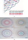 |
Figure 20 Gielis curves created with an HP7475A plotter [19]. (a) Details for a polygon with m = 43/10 with different colours for different exponents. (b) The complete curves. |
Having a Pythagorean compact analytic description for both shape and curvature for a wide range of shapes allows for a generalization of the notion of curvature. In [11] a new measure of curvature was introduced, directly related to the shape itself, using Gielis curves as osculating curves, as a generalization of studying curvature with circles.
Rational Gielis curves, R-functions and Flat tori
Rational Gielis curves
The self-intersecting curves for any rational m lead to various sectors in the polygons or cross sections of the GML body (Fig. 21). Figures 21a and 21c have three zones, while Figure 21b has four different zones of different shapes indicated with four different colours. In GML bodies, when cut and separated, these zones represent different bodies.
 |
Figure 21 Cutting pentagons from side to side. |
Self-intersecting Gielis curves can represent the same for planar graphs [20]. For rational m = p/q, the number of zones created in Gielis curves is determined by q, and the symmetry of the polygons/polygrams is determined by p. In Figure 22a, a 7/5 RGC or polygram is shown, having 7-symmetry, closing after five rotations if drawn in one line.
 |
Figure 22 (a) Different layers in Rational Gielis curves. (b) RGC for p = 5 and q = 4 with different zones defined [20]. |
In Figure 22a five different layers or zones can be defined in different shades of blue. Layers L0 to L4 are defined as a combination of layers from inside to outside and all layers have 7 maxima and 7 minima. A ray drawn from the centre 0 in any direction has multiple values indicated by I0 to I4 (red dots). When rotating the ray around the centre, the values of I0 defines the boundaries of L0 and the ray then sweeps the full area of L0. Values of I1 define the boundaries of L1, and here I0 and I1 coincide at maxima for L0 and at minima for L1. In the same way, values of Ii+1 define layer Li+1 .
The regular polygons and polygrams in the regular polygon and GML cutting can be considered as Gielis curves and can be transformed into the shapes in Figure 22b. Now, zones can be defined, not only as stacked layers L in Figure 22a, but as separate layers or combinations of layers. We define li as separate zones based on the different hues of blue zones in L0,…,4 in Figure 22a. Examples of separate zones or combinations are given in Figure 22b; clockwise, from upper left (with L0 = l0):
-
l1 is L1 − L0
-
l2 is L2 – L1
-
l3 is L3 – L2
-
l1 + l 2 is L2 – L0
The zones and the independent domains separated by lines correspond to self-intersecting Gielis curves. In Table 6 the results of cutting GML’s is compared with self-intersecting Gielis curves for symmetry m = 5 (Fig. 14).
GML versus Rational Gielis Curves RGC with m = p/q.
The order of cutting of GML or polygons is rearranged, showing the correspondence with self-intersecting curves. The number of independent figures and link number aligns with q and the number independent shapes that can be counted (separated by lines) is a function f of p.
In Figure 22b Layer L1 has five independent shapes, plus the central pentagon. Layer L2 has 11 (= 5 + 5 + 1) independent shapes or 2p + 1. In general f(p) = ap + 1, with a = 0, 1, 2, 3 and a + 1 = q. For a = 0, q = 1 the shapes close in one rotation, for all regular polygons. For q ≠ 1 the number of rotations to close the shapes is q and the shapes are then 2qπ-periodic. The zones l shown in Figure 22b, align with the self-intersecting curves in Table 6 with the pentagram m = 5/2 and the polygrams m = 5/3 and m = 5/4.
Boolean operations and R-functions
The number of independent shapes in Table 6 results from counting the isolated zones after cutting, delineated by lines. From a GML point of view, they are not independent, but are connected as sectors of a cut GML, according to a certain cutting process (Figs. 15 and 16 with link numbers). In Gielis curves, these independent figures can be connected into layers or zones (Figs. 22a and 22b) using R-functions [20]. This is a method to translate Boolean operations into geometrical figures, and allows for, amongst others, for blending or ensuring differentiability up to some order [20–23]. Basic Boolean operations can be used to define the different layers and separate sectors as in Figure 22 and these can be translated into geometric language [11, 20].
In Table 7 the most commonly used Boolean and associated R-functions are shown. The relationship to Lamé curves (from which the Gielis curves were derived) is clear via  (and special cases of Lamé curves; the superellipses |x1|
p + |x2|
p
and circle for p = 2): The use of exponents m/2 and 1⁄p converts Lamé curves into distances. In Table 7 we find
(and special cases of Lamé curves; the superellipses |x1|
p + |x2|
p
and circle for p = 2): The use of exponents m/2 and 1⁄p converts Lamé curves into distances. In Table 7 we find  or, a special Lamé curve
  , raised to exponent
  . This is the Pythagorean part distance
  raised to power m. The function
  has
has ![Mathematical equation: $ \left\langle {\left[{\left|{x}_1\right|}^p+{\left|{x}_2\right|}^p\right]}^{\frac{1}{p}}\right\rangle$](/articles/fopen/full_html/2020/01/fopen200013/fopen200013-eq90.gif) . Originally p is a positive integer but can now be any positive number p > 1 [20].
. Originally p is a positive integer but can now be any positive number p > 1 [20].
Examples of R-functions for the most common Boolean functions.
This leads to the remarkable fact that separated regions in RGC (and in polygrams in general) can be defined as coherent structures. Using R-functions, these operations are translated into geometry, whereby the different layers (Fig. 22a in blue) or different sectors (the red zones in Fig. 22b) are defined as single geometrical domains or combinations of single domains [20].
Knots and graphs
In this way we can connect seemingly unconnected zones in self-intersecting graphs in the very same way as the zones are connected when executing the cutting in 3D. Using R-functions the zones can be defined in planar graphs, which are connected as in 3D GML bodies. In GML bodies the resulting figures form separate bodies and in cross sections they show up as differently coloured, separated zones. In planar polygons, they can be connected via R-functions, but also by drawing graphs occurring in the cut polygons. Consider for example Figure 23. The boundaries of the yellow zones are defined by the circumscribing pentagon and by the inscribed pentagram (enclosing the brown and grey zone). Connecting the yellow zones, by using the boundaries of the innermost pentagram in grey, and considering only the boundaries, a graph is obtained.
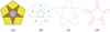 |
Figure 23 (a) Cross section of |

The boundaries of zones 1–5 (individual zones separated by small perpendicular blue lines), and connected by green highlighted lines, form a graph. This graph can be also obtained starting from the uppermost vertex of the inner pentagon with green highlighted sides, going around sector S1, then continuing along the green line to enclose S5, then to S4, then S3, and S2, ending this graph exactly at the upper vertex where the trajectory started. The same can be done for the brown sectors, and for the grey pentagon.
The boundary of graph enclosing the inner pentagon closes in one rotation, while the other two graphs self-intersect. These graphs are homeomorphic to the planar projection of a 51 knot (or RGC with m = 5/2) Figure 23c , or to Figure 23d .
These graphs also relate to the process of cutting GML in the following way. When cutting GML with a pentagonal cross section (as example), according to S1,3 cut, case BII, the result is a Link-3 of three separate bodies. The inner body is pentagonal, the second body has a triangular cross section and the outer one has a quadrangular cross section. In Figure 24 it is indicated how these bodies GML3, GML4 and GML5 are twisted. For ω = 1 and j = 0 = q the result is that the GML5 body is twisted 25 times (five full rotations), the GML3 body is twisted 27 times (nine full rotations), and the GML4 body is twisted 36 times (also nine full rotations). The overall structure is a link of 3 bodies, one of which (GML5) is the unknot with circle as basic line, while GML3, is a 51 knot, with the pentagram (or RGC with m = 5/2) as basic line.
The study of GML bodies and surfaces revealed complicated structures on interlinked bodies with knot structures, in particular the simplest knots k/2 (with k integer) or torus knots. These results also appear in the methodology of cutting planar regular m-polygons and in the methodology of self-intersecting Gielis curves and graphs (at least for ω = 1 and j = 0 = q as in the B II case in Fig. 24).
As a consequence, when cutting m-regular polygons, the link number and knot characteristics of the original GML from which they were cut can be found, counting the number of independent sectors, their shape and coherence as layers. Their coherence is established via R-functions, named after the Ukranian mathematician V.L. Ravchev (1926–2005).
Galilei, Euler, Catalan and Cayley
The problem of dividing m-polygons with non-crossing diagonals
Euler considered the following problem: in how many ways can one divide a polygon into triangles, in such a way that diagonals do not cross, i.e. similar to cutting with non-crossing knives [24]. For a pentagon using two diagonals this gives a total of five possibilities (Fig. 25). For a square, only two diagonals are possible.
 |
Figure 25 Five ways of cutting a pentagon, with diagonal knives. |
In the case of a pentagon, the cuts that are allowed are symmetric ones, VV1,2 and VV1,3. Using diagonals means vertex-to-vertex cuts and using the same notation as before these cuts are VV1,3 and VV2,4 in the square, giving two possibilities (Fig. 26a). The upper square gives VV1,3 (or VV2,4) while the lower one gives both possibilities in superposition. In the case of a pentagon, VV1,3 and VV1,4 diagonal knives (section “Chordal and radial knives”) can be used. For the GML case they are symmetrical, but for the Euler problem, they are different (Fig. 25). In Figure 26b, in the lower pentagon, all possible cuts are given with VV1,3 and VV1,4, starting from all five vertices. So the number of possible ways of cutting is 5. The lower pentagonal figure in Figure 26b can be considered as a composition of all VVi,i+2 and VVi,i+3 cuts of Figure 25.
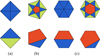 |
Figure 26 Cutting (a) square, (b) pentagon and (c) hexagon with diagonal knives. |
 |
Figure 27 Fourteen ways of cutting a hexagon, with non-crossing diagonals. |
In the hexagon (Fig. 26c) the possible cuts are also related to VVi,i+2 and VVi,i+3 cuts, and the total number of possibilities, is obtained when superposing the two lower hexagons. Possible cuts with VVi,i+3 and VVi,i+2 give the lower left and lower right hexagon, respectively. The number of possible cuts is 14 and the superposition of the lower two hexagons gives all possibilities. In other words, by superposition of the two hexagons, all possible individual paths for the Euler problem can be traced.
If one observes the upper row Figure 26c, a division by a VV1,3 cut (divisor 1) gives a triangle and a pentagon. The latter can be divided then into triangles, by VV1,4 and VV1,5 cuts. In Figure 26c, a VV1,4 divides the hexagon into two quadrilaterals, which can further be cut along their diagonals. This shows that this can be considered as a recursive procedure.
In heptagons VVi,i+2 and VVi,i+3 cuts are possible, and again, the superposition of the two lower figures in Figure 28 left, would give all possibilities. For octagons, VVi,i+2, VVi,i+3 and VVi,i+4 are possible diagonals. Overlaying all three lower octagons would give all possible solutions. In Figure 28 this is shown for the octagon, leading to 132 different possibilities.
 |
Figure 28 Cutting heptagons and octagons with diagonal knives. |
With superposition of the figures, diagonal knives seem to cross, but this is only superficially so, since the operations are carried out independently in GML rotating through one fixed knife. The question or problem that could be asked is the following:
Describe all possible ways of cutting m-polygons into triangles by using the allowed VV cuts. This can be carried out in 3D by using one knife each to cut the bodies. Each of the cuts corresponds to d-knives. The results will be the lower rows of polygons in Figures 26 and 28. Superposition of figures will give all possible paths.
The solution will be obtained in one operation if the process is executed in 3D by using three fixed knives simultaneously (example for the hexagon) if one moves a GML body through the knives.
Euler, Segner, Lamé and Catalan
The total number of possible cuttings with non-crossing knives of an m-gon, the problem originally studied by Euler [24, 25] is given in Table 8 for m = 5, … 10. The number r in the second row gives with the number of vertices r + 2, starting from r = 3, for a pentagon. This sequence of numbers, starting 1, 2, 5, 14, 42, … are Catalan numbers, which play a very important role in many fields of mathematics. The number r in Table 8 is the position in the row of Catalan numbers that start with 1 and 2.
Possible cuts for m-gons.
Euler found a solution to the problem in 1751. Euler’s number of possibilities Em:
 (14)
(14)
In 1758 the Hungarian mathematician Segner found a recursive formula. Let the vertices of any convex m-gon be 1, 2, 3,…, m. The triangle ∆1rm divides the polygons into an r-gon and an m + 1−r gon (Fig. 29). From this Segner’s recursive formula follows for (E2 = 1):
 (15)
(15)
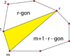 |
Figure 29 Dividing an m-gon into a triangle, r-gon and (m + 1 − r)-gon. |
For his newly established journal Joseph Liouville in 1838 asked proofs to combine the solution of Euler and the recursive one of Segner. Liouville published the geometric proof of Gabriel Lamé as the most elegant [26]. Later the same journal published solutions of Olinde Rodrigues and Eugene Catalan. They linked the sequence of numbers to combinatorial problems, for example the way in which a sequence of operations can be carried out using brackets. A recent book collects over 200 problems and questions in which Catalan numbers appear [27].
Euler, Liouville and Cayley
This is related to many other problems, which has involved many important mathematicians, such as Euler, Liouville and Cayley. One example: For m equally spaced points and all possible connections/diagonals drawn how many separate parts result? Examples are given in Figure 30 and the answer is OEIS A006533. The drawings once more correspond to our overlayed figures. It is possible to draw figures for any m via https://oeis.org/A006561/a006561.html.
 |
Figure 30 Original drawings of Jos Meeus. For m = n = 5 the original Pythagorean pentagon and pentagram result. |
For even m, diagonals of opposite points cross in the centre, while for odd m a central m-polygon is created, with the same shape as the original polygon, but rotated relative to the original polygon (Fig. 31). In GML/planar polygon strategy, diagonals through the centre can be created for odd m, by using a vertex to side cut, in particular a vertex to the middle of the opposite side, as for example in a pentagon. This is directly related to Table 6 and the sectors and layers in Rational Gielis Curves (RGC; section “Rational Gielis curves, R-functions and Flat tori”).
 |
Figure 31 Diagonals through centre for (VV1;m+2/2 cuts) and central m-polygons created for all other VV cuts. For m = 6, 8, 10. |
Cayley’s coloured partitions
A more general question on coloured partitions of a convex polygon by non-crossing diagonals was initiated by Cayley. For any positive integers a and b, all coloured partitions made by non-crossing diagonals of a convex polygons into polygons, whose number of sides is congruent to a modulo b can be obtained by recurrence relations and an explicit representation in terms of partial Bell polynomials [28]. Other relations can be found with Motzkin numbers and Dyke paths. This is very much related to the Euler problem in section “The Problem of Dividing m-polygons with Non-crossing Diagonals” and Figure 27, whereby the inscribed convex polygons reduce the number of vertices on the original polygons. In Figure 32 all paths of such inscribed polygons can be traced.
 |
Figure 32 Rational Gielis Curves with m = 8/2, 8/3 and m = 10/2, 10/3, 10/4, 10/1. |
Galilei, cycloids and clams
The non-crossing diagonals also appear in a problem of rolling polygons. If a polygon is rolled on a line the vertices form a polygonal arch. If one wants to compute the area under the polygonal arch this can be done by forming sets of blue, green and pink triangles in Figure 33. These can be arranged in the original polygon and this proves that the area under the polygonal arch is three times the area of the generating polygon [29]. The arrangement of the triangles in the polygons is one of the solutions of the Euler problem of cutting a polygon with non-crossing diagonals.
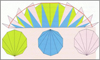 |
Figure 33 Determining the area under a polygonal arch. |
As a corollary, the area under a cycloid, generated by a fixed point on the circle as the rolling curve is three times the area of the circle. This corollary implicitly assumes that the number of sides of the polygon increases to infinity, with the circle as the limiting case.
With Gielis transformations however, we can keep the symmetry of the polygons fixed and morph them into circles by changing the exponents in order to have the transformation equal 1, i.e. exponents n are 2, the Pythagorean case. Piecewise linear and continuous are seamlessly combined.
If one considers the diagonals starting from the top in the blue polygon in Figure 33, the vertices represent the points reached by a ball, either dropped (central diagonal) or rolling off an inclined plane, in a fixed amount of time t1. Figure 34a is a figure from Galileo Galilei’s famous book, in which he discusses the phenomenon of a ball under friction and the force of gravitation [30]. Points E, G and I are points reached after a time t1. The greater circle, with points B, H and F is the locus for all points that are reached by a ball at a time t2 > t1. In nature such phenomena are observed in growth patterns in bivalve mollusks (Figs. 34b and 34c), and plant leaves as already observed in the original book Inventing the Circle [10]. So in some sense, we have come full circle after almost two decades.
 |
Figure 34 (a) Galilei’s original figure, (b and c) growth rings in shells. |
GML and Gielis curves as connectors
The theory of Generalized Möbius-Listing surfaces and bodies had been merged earlier with Gielis curves, either as cross section or as basic line. In the sections Expositio and Determinatio , it is shown that the connection between GML and planar Gielis curves runs much deeper, unveiling the relation between planar geometry, conic sections, GML surfaces and bodies, torus knots and planar knot projections, Flatland and branes, and more, and a wide range of methods and problems based on groups and equidistant points on a circle, revealing deep connections and equivalency of geometrical, arithmetical, logical, geometric-logical, combinatorial and algebraic methods.
In particular, a 3D problem can be solved by planar geometry but the problem of cutting GML bodies and surfaces is more general than related problems of non-crossing diagonals, or the number of sectors when connecting equally spaced points on a circle. Rotation allows for starting with one cut only and repeating this procedure, to find all possibilities of cutting. With rotation and scaling, VV cuts (classical diagonals) can become VS and SS cuts, or any possible cut dividing the m-polygon in exactly two parts with one knife. Solving the general case will allow to consider many other mathematical problems as parts of the general solution.
Constructio
Cutting a regular polygon
Consider a regular m-polygon. Vertices and sides are numbered from 1 to m. In Figure 35 the example of a pentagon is shown.
 |
Figure 35 Numbering of pentagon, vertices in blue, sides in red. |
A regular m-polygon can be cut in various ways, from vertex to vertex (notation VVij, e.g. VV1,3 from vertex 1 to vertex 3), from vertex to side (notation VSik, e.g. VS1,3 from vertex 1 to side 3), or from side to side (notation SSkl, e.g. SS1,3 from side 1 to side 3). VVmax, VSmax and SSmax are the cuts from and to vertices or sides with maximal separation (max is not necessarily the longest length). For example in Figure 35 VVmax = VV1,3 = VV1,4; VSmax = VS1,3 through the centre, and SSmax = SS1,3. If the line in SSmax cuts side 3 in the middle, and the cut of side 1 is moved to vertex 1, then SSmax can be made arbitrarily close to VSmax = VS1,3.
The following general facts can be observed in Figure 36:
-
In a polygon for even m, VVmax goes through the centre of the polygon (m = 6), and in a polygon for odd m, VSmax goes through the centre, crossing the side opposite the vertex in the middle (m = 7).
-
Going from a regular m-polygon to a (m + 1)-polygon introduces one extra vertex and one extra side. From m = 4 to m = 5 a line converts into a wedge of VV1,3 = VV1,4, giving one extra vertex and one extra side. Considering VSmax a wedge is created in m = even polygons (m = 8), and one line (through the centre) in m = odd polygons (m = 7, m = 9)
-
In m = 10, all cuts or diagonals are drawn from one vertex. Besides the VVmax the other VV cuts are two by two symmetrical (solid and dashed lines). In the case of m = odd, the same can be said for VS cuts (m = 7).
-
A single cut divides an m-polygon into two parts, which are defined by their shape and number of vertices and sides. In m = 4 the square is divided by the red diagonal into two triangles. In m = 6 the hexagon is divided into two equal quadrilaterals or trapezoids. In m = 11 the polygons is divided into an octagonal shape with 8 vertices, and a pentagonal shape with 5 vertices.
 |
Figure 36 Understanding modes of cutting. |
Cutting and divisors of m
There is a definite relation between the ways of cutting and the number of divisors of m. In Figure 36, m = 11, a VV1,5 cut is related to the smallest divisor of m, dmin = 1. For m = 12:
-
VV1,4 cut (dark blue dashed line), is repeated as VV4,7 and as VV7,10 and VV10,1. In fact, the latter cuts are obtained from the original VV1,4 cut (blue dashed line) by a rotation by
 . This gives a square, related to divisor 4.
 -
VV1,5 cut (blue solid line), is repeated as VV5,9 and as VV9,1. In fact, the latter cuts are obtained from the original VV1,5 cut (blue solid line) by a rotation by
 . This gives a triangle, related to divisor 3.
 -
VV1,3 cut will give a hexagon. If this is cut is repeated 6 times over an angle of
 , related to divisor 6.
 -
VV1,2 cut does not divide the polygon, but coincides with the original side 1. Rotation this by
 will give the original dodecagon. An inscribed dodecagon is obtained via a SS1,2 cut, rotated twelve times by
  . Both cases are related to dmax = 12.
In m = 4 the upper blue line is a SS1,2 cut from side 1 to side 2. When rotated by 180° the lower blue line is obtained, for the second smallest divisor d2 = 2.
The inscribed figures (triangle and square in m = 12) close in one rotation but this can be generalized, for  with p, q rational numbers and relative prime.
-
In m = 5 the sequence VV1,3, VV3,5, VV5,2, VV2,4, VV4,1 will generate a pentagram in the pentagon, i.e. a figure that closes in two rotations, having five angles that are spaced
 apart. This generates the classic Pythagorean pentagram that led to the discovery of irrational numbers and the golden ratio, corresponding to a RGC with m = 5/2.
 -
In m = 7 the sequence VV1,3, VV3,5, VV5,7, VV7,2, VV2,4, VV4,6, VV6,1 generates a heptagram, closing in two rotations, corresponding to a RGC with
 .
. -
Also in m = 7 the sequence VV1,4, VV4,7, VV7,3, VV3,6, VV6,2, VV2,5, VV5,1 generates a heptagram, closing in three rotations, corresponding to a RGC with
 .
.
Rotations and scaling
For m = 16 results of cutting with dm knives for divisors 2, 4, 8 and 16 are shown in Figure 37. They are rotations of the d1 knife.
 |
Figure 37 Cutting with di knives (d2 = 2, d3 = 4, d4 = 8, d5 = 16) and the resulting sectors. |
The relation of divisors and rotations show that VV and SS cuts can be transformed into each other by rotations:
-
In m = 6, the VVmax = VV1,4 cut or diagonal can be rotated every 60° and all diagonals meet in the centre (result is 6 diagonals that coincide 2 by 2) (Fig. 38).

Figure 38 Converting VVmax into SS cut through centre of the sides by rotation.
-
This shape can then be rotated by 30°, resulting in SSmax. The rotation can in fact be done for any angle.
There are many ways in which the figures can be transformed into the other figures, using rotation and scaling. A first example sequence of rotations and scaling could be:
-
If the red square in Figure 39f is rotated by 45° the result is 39c.

Figure 39 Ways of cutting square.
-
If the red square in Figure 39c is scaled to size zero, 39d results.
-
If the cross in Figure 39d is rotated by 45° the result is Figure 39a .
A second example in Figure 39:
-
If the red square in f is scaled to a larger size, e results; when it is scaled to a smaller size g results.
-
When the inscribed figure in g is rotated so that one of the sides of the small yellow triangles ends in a vertex, we obtain b.
This shows that all figures can be considered as transformations of an inscribed square (and in general the inscribed m-polygon inside an m-polygon). The analytic representation of the di-knife was given in section “GML versus Polygon Cutting with 1 or m Knives” (Eqs. (12) and (13)) [8].
The way of cutting determines the final result
In Figure 39 from left to right, all possible cuts are shown for a square
-
a. One case of VV cut, with two VVmax diagonals
-
b. One case of VS cut, with a VS1,2 cut and its rotations over
 . In total three different shapes are created. Four green triangles, four blue quadrilaterals and one red square. The smaller red square can be considered as the inscribed square rotated and scaled to smaller size.
 -
c and d. Two cases of SSmax = SS1,3 cuts and rotations. One SS cut does not pass through the centre (c.) and the other one passes through the centre (d). The former creates three different sets of quadrilaterals indicated by different colours. The latter creates four different squares. (In GML in d. these four different squares form one body, and in c. each of the coloured zones creates 3 separated bodies)
-
Three cases of SS1,2 cuts (e, f, g). It is clear that the result depends on where the cut is made. The middle figure f. is the inscribed square, while e. and g. are scaled versions (larger and smaller, without rotation).
-
This also generates different shapes. In e. four triangles and one octagon; in f. four triangles and one square and in g. one set of four triangles, one set of four pentagons and a central square. Again, in GML and in rational Gielis curves RGC they will form different bodies or layers.
The same logic is applied to hexagons in Figure 40, with more possibilities of cutting, namely two VV cuts, two VS cuts and eight SS cuts.
 |
Figure 40 Hexagon cutting. |
Inheritance of possible cuts for different divisors
In Figure 41 VV and VS cuts are shown for m = 4, 6. A square has three divisors, so 3 rows; for the hexagon there are four rows corresponding to 4 divisors. For m prime only 2 rows result, for divisors m and 1.
-
For even m the vertical columns of square and hexagon in Figure 41 show that the possible cuts are the same for all divisors, as the result of rotating cut 1 over the relevant angle, related to divisor. The identification of vertices and of the knife (e.g. for d2 = 2 lower row Fig. 41) links the cutting of m-polygons to cutting of
 bodies.
 -
For odd m (in case of pentagon in Fig. 42), the VV cuts are inherited from cut 1 via rotations. This is not the case for the VS cuts of the pentagon in Figure 42. However, one figure is missing in the upper row, namely the VS cut not through the centre. If this figure is also considered, then also for the pentagon the number of cuts is fully inherited for the two divisors, as in the case of the even m.

Figure 41 VV and VS cuts of square and hexagon.

Figure 42 All possible cuttings of a pentagon via VV, VS and SS cuts.
-
The reason why in Figure 42 for the pentagon (and in general for any odd m) only one figure is shown for VS (the cut through the centre) is that the number of sectors and the number of vertices and sides of the resulting polygons remains the same. In the case of the pentagon and VS1,3 = VSmax, two quadrilateral figures are created, whether or not the cut goes through the centre. The quadrilateral shapes share the topological characteristic of four vertices and four sides.
-
In case of the VS1,3 = VSmax cut going through the centre, the two quadrilateral shapes have also the exactly same shape, a geometrical characteristic. If VS1,3 ≠ VSmax , i.e. not going through the centre, then the geometrical shape of the two quadrilaterals is different.
So, if this geometrical characteristic is considered, also for divisor 1 or one cut, two different shapes need to be considered, whereby the two shapes are different or the same. In the topological case, these two shapes reduce to one shape as in Figure 42. The same line of reasoning can be considered for SS cuts, where in Figure 42 there are 2 line cuts in upper row versus 8 in the lower row.
In general, starting from the maximum divisor, or max cuts equal to m, for other divisors the number of possibilities is inherited precisely, in the geometrical sense.
d-knives and projective geometry
The analytic definition of d-knife is a construction, with m straight lines ([8], section “Defining knives for all divisors”)

The precise cutting with a di-knife can also be considered as a projection of a shape with symmetry m or one of the divisors of m, onto the basic shape of the cross section of the GML with symmetry m, along a cone with the same cross section (Fig. 43). Cutting with a dm-knife is equivalent to projecting an m-regular polygon onto an m-regular polygon with zooming parameter δ. In Figure 43 the projection of a red square onto a green square (the basic one) is shown. At the top of the pyramid, the red square reduces to one point and the blue zone narrows to lines, as in Figures 39c and 39d.
 |
Figure 43 Projective equivalence with cutting with di knife for squares dm = 4. |
For the smallest divisor 1 the cut is with one knife, and this cut can be repeated by rotation as in Figure 37 for other divisors. For even numbers the second smallest divisor d2 = 2 and a rectangle is projected which at the top of the pyramid also reduces to a line (compare Fig. 41 lower row), and so on. This projection corresponds to the dilation parameter δ. Rotation parameter α corresponds to a rotation of the prismatic pyramid relative to the base polygon.
The number of independent objects after cutting
When cutting m-regular polygons or GML bodies (or more generally Generalized Rotating and Twisting  surfaces and bodies, whereby the basic line is a Gielis curve with m rational), this leads to a number of independent sectors in the plane cross-sections. Tables 9 and 10 give for some even and odd values of m all possibilities:
-
di, i = 1,2, …, m are different divisors of the number m. N is the number of different nontrivial (di ≠ 1, m) divisors of the number m.
-
If m = 2k + 1 then all divisors di, i = 1, 2, …, N of m are odd numbers.
-
If m = 2k some of its divisors di, i = 1, 2, …, N may be odd.
Example cuts of  bodies for odd m = 3, 5, 9, 27.
Example cuts of  bodies for even m = 4, 6, 8, 10, 24.
Remark: For odd m a complete correspondence is found with Rational Gielis Curves for VV-cuts. For example for m = 5 (section “Rational Gielis curves, R-functions and Flat tori” and Tab. 6): if 
 the number of independent shapes are 6, 11 and 16 (for p = 5, resp. p + 1, 2p + 1 and 3p + 1).
Using radial knives
The Möbius phenomenon only occurs for m even, when the knife cuts through the centre, since only then congruent figures are obtained through cutting that can be connected throughout with a twist. Going through the centre is an important condition, but whether the cuts are VV, VS or SS is less important: Möbius phenomena can occur in all cases. This Möbius phenomenon never occurs for m = odd; while then congruent figures may be obtained, they only have mirror symmetry, not rotational.
The main condition, congruent figures and rotational symmetry, is achieved when using radial knives (see Sect. “Chordal and Radial knives”), emanating from the centre C of the figure, to the perimeter, so CV or CS cuts result with the length of the knife half compared to the previous knives. In this case the Möbius phenomenon can be achieved in all cases, irrespective whether m is odd or even. The word knife can be substituted by other words, like secants, diagonals, rays and chords, but has the advantage that the separated zones can actually be separated.
Demonstratio
The geometrical solution
The total number of ways of cutting an m-polygon according to the rules described above with d-knives for the geometrical case, for m = even and m= odd respectively is as follows: VV, VS and SS cuts increase from by 1, 1 and 3 respectively from a given even or odd number to the next even or odd number. As a result, the total number of ways of cutting using a dm knife increases by 5 to each subsequent even or odd number (Tab. 11, Subtotal), which gives the sequence (2), 2, 7, 7, 12, 12, 22, 22, 27, 27, 32, 32, 37, 37 … for m = 2, 3, 4, 5 … 15. Taking sums the sequence 4, 14, 24, 34, 44, 54, 64, 74 … results, which is monotonically increasing.
Number of possible cuts for even and odd m.
Since the number of possibilities is determined by d1 and dm and is inherited by the other divisors given identification of vertices and knives (Fig. 44 for divisors 1, 2 and 6 in a hexagon), the total number is then the subtotal times the number of divisors. The identification links planar geometry to 3D  bodies. If one follows the d1-knife along the basic line of the
  body, the different positions of the knives indicated by arrows in Figure 44 for d1 function as a clock, relative to the torus circumscribing the
  body. For other knives the clock arithmetic is the same, albeit with more hands.
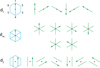 |
Figure 44 Inheritance from d1 by all d-knives through identification and direction of knives. |
Table 12 gives the product of the subtotals with positive integers. Entries in rows can be computed as un = un−1 + un−2 − un−3, with u0 = 2 for even and u0 = 3 for odd numbers. In bold red are the totals of Table 11 for m odd and in green for m even.
The number of possible cuts can be given by a recurrence formula. For Nm, the number of ways of cutting an m-gon for one divisor, whereby  stands for the number of SS cuts for m and
  for the number of SS cuts for the polygon with (m − 2) (i.e. the previous odd or even number) and with k a natural number.
-
For even m (= 2k):
 (1a).
(1a). -
For odd m (= 2k + 1):
 (1b).
(1b).
If the number of SS cuts is kept separate, taking into account the step +3, this part of the general formula is recursive. Since  , it follows that
  = …
= …
Because of the exact inheritance for the geometrical case the total number of ways of cutting for all divisors is then the above formula times the number of divisors  of a number m.
Theorem 1. (the geometrical solution).
The total number of different ways of cutting an m-polygon
 is the number of 1 or m cuts, times the number of divisors of m.
-
For even m (= 2k):
-
For odd m (= 2k + 1):
When considering polygons with convex sides, VVi,i+1 are possible, so the number of cuts increases by m. When knives are used to cut a circle from equally spaced points, the VVi,i+1cuts need to be added, in particular m cuts.
-
For even m (= 2k):
 (2a)
(2a) -
For odd m (= 2k + 1):
 (2b)
(2b)
The topological solution
The number of ways of cutting an m-polygon according to the rules for the topological solutions is given in Table 13 for for m = 3, 4, …, 16. Appendix graphically shows all possibilities for for m =6, 7, 8, 9, 10. From this follows Theorem 2 (the atopological solution).
All possible cuttings for m-regular polygons for m = 3, 4, …, 16.
Theorem 2. (the topological solution)
If m = 2k + 1 and has N nontrivial divisors d2, d3
… dN+1
and d1
≡ 1, dN+2
≡ dm
≡ m, then the number of all possible variants of cutting of
 bodies is
![Mathematical equation: $$ {\mathrm{\Xi }}_m^{{top}}=8k+1+3{Nk}+\sum_{i=2}^{N+1}\left[\frac{k}{{d}_i}\right]+2N $$](/articles/fopen/full_html/2020/01/fopen200013/fopen200013-eq124.gif)
If m =2k and has N nontrivial divisors d2,d3 … dN+1 and d1 ≡ 1, dN+1 ≡ dm ≡ m, then the number of all possible variants of cutting of  bodies is
![Mathematical equation: $$ {\mathrm{\Xi }}_m^{{top}}=8k-5+3{Nk}+\sum_{i=2}^{N+1}\left[\frac{k-1}{{d}_i}\right]-N $$](/articles/fopen/full_html/2020/01/fopen200013/fopen200013-eq126.gif)
This is in a slightly different form compared to Theorem 1:  depending on whether the total number of variants is expressed in terms of total number of divisors or total number of non-trivial divisors N (excluding d1 and dm).
The complete proof of Theorem 2 will be given in a separate paper. It is based on the fundamental facts from the theory of cyclic groups with a finite number of elements (m);
-
The number of cyclic subgroups is the number (N) of nontrivial divisors of m.
-
The number of elements in each subgroup is the number of transactions and equal to the gcd(m, i).
-
The number of cuts is either 3 or 1, (3 or 1 mod 8) and this is determined by the property of the subgroup and the property of the cut line – i.e. when the number of cuts is three, then the ends of the survey line lie on the same strings of the initial polygon, except for the case when
![Mathematical equation: $ k=\left[\raisebox{1ex}{$m$}\!\left/ \!\raisebox{-1ex}{$2$}\right.\right]+1$](/articles/fopen/full_html/2020/01/fopen200013/fopen200013-eq128.gif) .
. -
If
![Mathematical equation: $ k=\left[\raisebox{1ex}{$m$}\!\left/ \!\raisebox{-1ex}{$2$}\right.\right]+1\enspace $](/articles/fopen/full_html/2020/01/fopen200013/fopen200013-eq129.gif) and for an odd number m the number of cuts is 5, and for even m the number of cuts is 2. This is determined by the property of the subgroup and the property of the cut line. In the latter case m = 2k an important role is played by the rotational symmetry.
and for an odd number m the number of cuts is 5, and for even m the number of cuts is 2. This is determined by the property of the subgroup and the property of the cut line. In the latter case m = 2k an important role is played by the rotational symmetry.
Number of independent bodies or zones
Theorem 3.
The number of independent objects depends on 1) the type of cut, 2) the divisor or di-knife, and 3) the parity of m and its divisors. For odd or even m the number of possible independent objects appearing after different cuts of m-polygons and
 bodies with di-knives is given in
Table 14
for odd and even m.
bodies with di-knives is given in
Table 14
for odd and even m.
Various cuts of m-polygons and  bodies with di-knives for odd and even m.
2·di
* – When di
* is an even number, the di-knives turn into
 -knives and therefore the result is as if it were acting similar to the
 knives.
Möbius phenomena
Theorem 4
In the cutting of GML bodies with chordal knives, the Möbius phenomenon with one resulting body and link number 1 can appear only for m even and when the knife cuts through the centre. In the cutting of GML bodies the Möbius phenomenon can appear for both m odd and m, when the knife is a radial knife, a ray starting at the centre of the polygon.
The radial knife is actually the position vector. This acts as the hand of a clock with discrete ticks (Fig. 45) but with continuous movement within a  body, keeping a fixed direction from centre to the vertex. During this continuous movement, the various vertices of the polygon coincide with the upper circle in a torus in discrete steps. The tip of the position vector traces out a toroidal line, wound around the torus, now in a continuous way.
 |
Figure 45 Radial knife or position vector. |
Conclusio
Möbius before and after Möbius
The Möbius strip is an icon of mathematics. It was named after the German mathematician Möbius, but was known already 2 millenia ago (Fig. 46). This “twisted cylinder” is obtained by giving one end of a rectangular strip of paper a twist before joining both ends. Simple as this may seem Möbius strips are one-sided, non-orientable surfaces with some counterintuitive properties. Tracing out a path on a Möbius strip will show that it has only one side and the whole strip can be painted in one color without lifting the paint brush. If some form of identification is done along the central line before joining, one will find that orientations are reversed after rejoining. Johann-Benedict Listing (1808–1882) and August Ferdinand Möbius (1790–1868) discovered these remarkable objects in the mid-nineteenth century. The name Topology – the study of shape characteristics independent of measuring – was used first by Listing. While topology is a branch of geometry, Listing chose the name topology to avoid reference to measurements and referred to “Modalität und Quantität” (modality and quantity) to distinguish between shape and magnitude.
In On Growth and Form, D’Arcy Thompson [32] summarized the field and its initial historical development: “...in this study of a segmenting egg we are on the verge of a subject adumbrated by Leibniz, studied more deeply by Euler, and greatly developed of recent years. It is the Geometria situs of Gauss, the Analysis situs of Riemann, the Theory of Partitions of Cayley, of Spatial Complexes or Topology of Johann Benedict Listing... Leibniz has pointed out there was room for an analysis of mere position, apart from magnitude: “Je croy qu’il nous faut encor une autre analyse, qui nous exprime directement situm, comme l’Algèbre exprime magnitudinem”. .. Leibniz used it to explain the game of solitaire, Euler to explain the knight’s move on the chessboard or the routes over the bridges of a town. Vandermonde created a géometrie de tissage, which Leibniz himself had foreseen, to describe the intricate complexity of interwoven threads in a satin or brocade. Listing, in a famous paper, admired by Maxwell, Cayley and Tait, gave a new name to this new “algorithm”, and shewed its application to the curvature of a twining stem or tendril, the aestivation of a flower, the spiral of a snail-shell, the scales on a fir-cone, and many common things. The theory of “spatial complexes”, as illustrated especially by knots, is a large part of the subject”. There are many things to which the new Geometria Situs could be applied.
Geometrical topology
Analysis situs or topology developed over many centuries, and has developed into highly abstract mathematics at one extreme and into various educational tools for displaying the magic of mathematics at the other. Möbius bands are icons of mathematics [33], and so are knots and links. It is also linked to geometry, in particular, the inner geometry of surfaces, starting with Gauss’ Theorema Egregium. Indeed, a torus can be constructed topologically by folding a piece of paper into a cylinder and connecting the ends. For this reason the intrinsic geometry of the torus and the piece of paper (exemplifying part of the plane) is the same, and hence the torus is considered as a flat surface (in contrast to a sphere). In similar ways Möbius bands, Klein Bottles and Projective planes can be constructed by taking a piece of paper, identifying opposite sides and connecting those in the appropriate way. The projective plane is a disk to which a Möbius band is glued.
Nevertheless, these are recipes or instructions to generate surfaces, and one of the main lacunae in the geometry/topology distinction is the absence of general but simple analytic representations. Even the whole field of knots still only leads to tabulations, not classifications. Our analytic representations or equations substitute for “recipes” or “(computer) algorithms” to “generate” Möbius strips, tori, helices or more complex shapes. We no longer need all types of different parametrizations for different shapes, but we can combine these shapes now into single equations, allowing for continuous transformations from circle or sphere into any other shape, including knots and certain polyhedrons, irrespective of topological constraints.
In this sense transformations from sphere to torus e.g. with intermediates as ring, horn and spindle tori, or to knots are very natural, and continuous. The definition of a torus as S 1 × S 1, or fibre bundles with unit intervals as fibre over manifolds [34], or processes such as making holes and using surgery or pinching, can be approached from another, continuous geometric perspective. In this perspective shapes can be transformed into each other and cut into predictable substructures. The reduction of “recipes” to equations, with a concomitant reduction of shape complexity, has always led to progress in science. This “old kind of science” has been extremely valuable for mankind, from Greek mathematics to the present day. By focusing on some very elementary ideas, such as the Pythagorean structure of Gielis curves and Gaspard Monge’s idea of describing complex movements as superpositions of elementary ones for GML [35], highly complex structures and very many of the well-known shapes in mathematics can be described in very simple analytic representations. There are one-to-one mappings from one shape to the other, and these mappings are geometrical, at times violating the rules of topology, but at the same time bridging topology and geometry.
In our work we focused so far on the “forward” approach, but we believe that uniqueness results can be proven, so that from observing and counting complex structures it should be possible to reconstruct the original GML body or surfaces from which it was derived.
The general case of cutting GML
The generalization of Möbius ribbons to Generalized Möbius-Listing bodies and surfaces was initiated in the late nineties of last century [1]. The motivation was the fact that the solution of partial differential equations strongly depends on the topological properties of the domain on which the problem is considered. The first results were obtained on Möbius strips, giving a general solution for cutting of ribbons for any number of twisting and for any number of cuttings. Consequently the description was broadened to include surfaces and bodies and in the recent decade, classifications were also obtained for GML bodies and surfaces with convex cross-sections for symmetries m = 2, 3, 4, 5, 6.
These developments became possible by integrating GML and Gielis curves and bodies, a geometric transformation describing a very wide range of abstract and natural shapes. This integration made it possible to develop strategies to achieve a general classification for cutting of GML bodies of any symmetry, starting from cross sections that are m-regular polygons. The original problem could be reduced to the problem of cutting m-regular polygons with crossing diagonals or knives. With the proposed methods even the topological characteristics of the resulting bodies and surfaces and their link number can be found with the 2D strategy of cutting polygons.
Determining the number of variants after cutting has both geometrical and topological solutions, resulting in Theorems 1 and 2. These theorems not only give the precise number of variants after cutting, but also allow for determining the precise shape of the resulting bodies and their topology. Appendix gives all relevant graphics from m = 6 to m = 10. Theorem 3 gives the number of different objects resulting from specific ways of cutting, and from this one can count the connected zones in polygons or the link number after cutting of  bodies. It generalizes the cutting of polygons and partitions in the sense of Euler and Cayley, with VV cuts and diagonals. Because of these connections, combinatorial or other approaches could have been used, but the strategy of using planar geometry (as a reduction of a 3D problem), has the advantage of revealing many connections and a broad scope of applications, and the additional advantage of having a strong educational component.
Theorem 4 gives the precise conditions under which the Möbius phenomenon will occur for regular polygons with both odd and even symmetry m, when using radial knives. The radial knife is nothing but the position vector, which is static if defined as m-polygons, but dynamic using Gielis transformations, allowing to morph the polygon into circles, starfish and so on. The tip of the knife traces out a toroidal line on the circumscribing torus, whereas the knife itself describes a surface. When the  body is not closed, a generalized cylinder results. The generalized cylinder can also be a generalized cone. The tip of the arrow traces out a helix, but with m-symmetry. The arrow itself than traces out a surface, in particular a Riemann surface. If the arrow has a given depth (thickness in the direction of the cylinder), it will trace out a body or helical shell. If the arrow has a given depth in this case, it will trace out a shell body as observed in mollusc shells.
Future work
The results are obtained for regular polygons, but can easily be generalized. First, Gielis curves and curved knives greatly generalizes these results, for convex and concave domains. Second, knives can be the result of some optimization problem in convex geometry. Third, only one knife in one direction was used, but k-knives [3] with multiple parallel blades can be used to make multiple parallel cuts at once; in the extreme the knife can be a Cantor-knife, such that the resulting cut gives in cross section the Cantor continuum. Fourth, the definition of di-knives starts from d1-knife by i rotations with the centre of the polygon as centre of rotation, but different movements of d1-knives will give other results. One example is the Cremona construction of the cardioid, as envelope of a pencil of lines. This is realized with VV cuts of the type VVi,2i connecting n equally spaced points on the circle.
These results open up many new possible areas of research, in particular for a unified and general geometric framework for the study of natural phenomena in biology, chemistry and physics, both in the small and in the large. It also opens up many challenges.
In physical realisations Möbius bands will take on shapes, which are physically dependent, among others, on width, length and material [36]. Within the more general framework of  or cylinders with non-circular cross sections, the situation is very different. In the case of cylinders subjected to torsion, the cross sections are known to remain planar. The research of Adhémar Jean Claude Barré de Saint-Venant (1797–1886) on the torsion of prisms and non-circular rods [37] showed how the internal body is subjected to stress resulting in distorted, anticlastic cross sections (Figs. 47a and 47b). The lines that remain in-plane are VV and SSC cuts perpendicular to the sides for the square or
  cuts for the triangle. This phenomenon was observed in the horns of rams (Fig. 47c) [32]. The stresses and strains and the displacements (Fig. 47) connect shape and differential equations. Elasticity theory then enters the field, a wide research domain of elastic and prismatic cusped shells, plates and beams [38], (Fig. 1).
 |
Figure 47 Torsion of prisms with square (a) and triangular (b) cross-sections. Dotted lines are depressed regions and full lines are elevated parts of the cross sections. (c) Anticlastic surfaces in the horns of rams [32]. |
Precise knowledge of the domains is essential for solving boundary value problems and this was precisely the motivation for the study of  surfaces and bodies (in particular, the starting point was the study of Saint-Venant’s Principle on complex domains). The same motivation underlies the development of R-functions [11, 22].
Our methods allow for the precise description of a wide variety of domains in a uniform geometric way, based on GML/GRT and plane geometry. With Gielis transformations continuous transformations among domains are added. This leads to naturally adapted coordinate systems on which boundary value problems can be solved, which is the essence of mathematical physics, according to Gabriel Lamé, who was also one of the main contributors to elasticity theory [37].
Appendix
All possible ways of cutting polygons (m = 6, 7, 8, 9, 10) with a chordal knife.
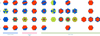 |
Figure 48 Hexagons (m = 6). |
 |
Figure 49 Heptagons (m = 7). |
 |
Figure 50 Octagons (m = 8). |
 |
Figure 51 Nonagons (m = 9). |
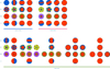 |
Figure 52 Decagons (m = 10). |
Labelling is from 1 to m for both vertices and sides. In earlier publications [1–6] numbering starts from 0 in the case of vertices.
The versine was used to measure curvedness in railroad tracks, by spanning a chord AB and measuring the distance CD from the chord to the track.
This argument can be used to proof the incommensurability between side and diagonal.
Or straight lines in a Poincaré disk.
References
- Tavkhelidze I (2001), On the some properties of one class of geometrical figures and lines. Reports of Enlarged Sessions of the Seminar of I. Vekua Institute of Applied Mathematics 16, 1, 35–38. [Google Scholar]
-
Gielis J, Tavkhelidze I, Ricci PE (2013), About “bulky” links generated by generalized Möbius-Listing bodies
 . J Math Sci 193, 3, 449–460.
[CrossRef]
[Google Scholar]
. J Math Sci 193, 3, 449–460.
[CrossRef]
[Google Scholar]
- Tavkhelidze I (2011), About connection of the generalized Möbius listing’s surfaces with sets of ribbon knots, in: Proceedings of Ukrainian Mathematical Congress S. 2, Topology and geometry – Kiev, pp. 117–129. [Google Scholar]
-
Tavkhelidze I, Cassisa C, Gielis J, Ricci PE (2013), About bulky links, generated by generalized Mobius-Listing’s bodies
 . Rendic Lincei Mat Appl 24, 11–3.
[Google Scholar]
. Rendic Lincei Mat Appl 24, 11–3.
[Google Scholar]
- Tavkhelidze I, Ricci PE (2017), Some properties of “bulky” links, generated by generalised Möbius–Listing’s bodies, in: Modeling in Mathematics, Atlantis Press, Paris, pp. 159–185. [Google Scholar]
- Pinelas S, Tavkhelidze I (2017), Analytic representation of generalized Möbius-listing’s bodies and classification of links appearing after their cut, in: International Conference on Differential & Difference Equations and Applications, Springer, Cham, pp. 477–493. [Google Scholar]
- Gielis J (2003), A generic geometric transformation that unifies a wide range of natural and abstract shapes. Am J Bot 90, 3, 333–338. [CrossRef] [PubMed] [Google Scholar]
-
Tavkhelidze I, Gielis J (2018), The process of cutting
 bodies with dm knives, in: Reports of the Enlarged Sessions of the Seminar of I. Vekua Institute of Applied Mathematics Vol. 32.
[Google Scholar]
bodies with dm knives, in: Reports of the Enlarged Sessions of the Seminar of I. Vekua Institute of Applied Mathematics Vol. 32.
[Google Scholar]
- Gielis J, Haesen S, Verstraelen L (2005), Universal shapes: from the supereggs of Piet Hein to the cosmic egg of George Lemaître. Kragujev J Math 28, 55–67. [Google Scholar]
- Gielis J (2001), Inventing the Circle, Geniaal, Antwerpen (2003), in: Dutch: De uitvinding van de Cirkel (2001), In Dutch. [Google Scholar]
- Gielis J (2017), The Geometrical Beauty of Plants, Atlantis-Springer. [CrossRef] [Google Scholar]
- Matsuura M (2015), Gielis’ superformula and regular polygons. J Geom 106, 2, 1–21. [CrossRef] [Google Scholar]
- Fougerolle YD, Gribok A, Foufou S, Truchetet F, Abidi MA (2006), Radial supershapes for solid modeling. J Comput Sci Technol 21, 2, 238–243. [Google Scholar]
- Gielis J, Natalini P, Ricci PE (2017), A note about generalized forms of the Gielis formula, in: Modeling in Mathematics, Atlantis Press, Paris, pp. 107–116. [Google Scholar]
- Abbott EA (1884), Flatland, A Romance of Many Dimensions. By A. Square, Seeley, London. [Google Scholar]
- Cutting bamboo poles [Google Scholar]
- Haesen S, Šebeković A, Verstraelen L (2003), Relations between intrinsic and extrinsic curvatures. Kragujevac J Math 25, 25, 139–145. [Google Scholar]
- Weisstein EW (2009), CRC Encyclopedia of Mathematics, CRC Press, USA. [Google Scholar]
- Nisley E (2016), Plotting like it’s 1999 – scrap to Superformula, Poughkeepsie ACM Chapter. [Google Scholar]
- Fougerolle Y, Truchetet F, Gielis J (2017), Potential fields of self intersecting Gielis curves for modeling and generalized blending techniques, in: Modeling in Mathematics, Atlantis Press, Paris, pp. 67–81. [Google Scholar]
- Shapiro V (2007), Semi-analytic geometry with R-functions. Acta Num 16, 239–303. [CrossRef] [Google Scholar]
- Rvachev V (1974), Methods of logic algebra in mathematical physics, Naukova Dumka, Kiev (in Russian). [Google Scholar]
- Rvachev VL, Rvachev VA (1979), Neklassicheskie metody teorii priblizhenij v kraevyh zadachah [Non-classical methods of approximation theory to boundary tasks], Naukova dumka Publ, Kiev. [Google Scholar]
- Euler L (1965), Leonhard Euler und Christian Goldbach, Briefwechsel 1729–1764, in: A.P. Juskevic, E. Winter (Eds.), , Akademie Verlag, Berlin. [Google Scholar]
- Euler L (1758–59), Novi Commentarii Academiae Scientarium Imperialis Petropolitanque 7, pp. 9–28. [Google Scholar]
- Lamé G (1838), Un polygone convex étant donné, de combien de manières peut-on le partager en triangles au moyen de diagonales? J Math Pure Appl 3, 505–507. [Google Scholar]
- Koshy T (2009), Catalan Numbers with Applications, Oxford University Press, New York. [Google Scholar]
- Birmajer D, Gil JB, Weiner MD (2017), Colored partitions of a convex polygon by noncrossing diagonals. Discrete Math 340, 4, 563–571. [Google Scholar]
- Mallinson PR (1998), Proof without words: Area under a polygonal arch. Math Mag 71, 2, 141–141. [CrossRef] [Google Scholar]
- Galilei G (1638), Dialogue concerning the two chief world systems. [Google Scholar]
- Cartwright JH, González DL (2016), Möbius strips before Möbius: Topological hints in ancient representations. Math Intell 38, 2, 69–76. [CrossRef] [Google Scholar]
- D’Arcy TW (1917), On growth and form, Cambridge University Press. [Google Scholar]
- Gielis J, Tavkelidze I, Caratelli D, Fougerolle Y, Ricci PE, Gerats T (2012), Bulky knots and links generated by cutting Generalized Möbius Listing bodies and applications in the natural sciences, in: Royal Academy of Flanders. Proceedings of Math Art Summit 2012, Brussels. [Google Scholar]
- Weeks JR (1985), The shape of space. How to visualize surfaces and three-dimensional manifolds, Marcel Dekker. Chapter 17 Bundles. [Google Scholar]
- Tavkhelidze I, Caratelli D, Gielis J, Ricci PE, Rogava M, Transirico M (2017), On a geometric model of bodies with “Complex” configuration and some movements, in: Modeling in Mathematics, Atlantis Press, Paris, pp. 129–158. [Google Scholar]
- Starostin EL, Van Der Heijden GHM (2007), The shape of a Möbius strip. Nat Mater 6, 8, 563. [CrossRef] [PubMed] [Google Scholar]
- Todhunter I (1893), The history of elasticity and of the Strength of Materials – from Galilei to the present time, Volume II Saint-Venant to Lord Kelvin, Part 1, Cambridge University Press. [Google Scholar]
- Vekua IN (1985), Shell theory: general methods of construction, Vol. 25, Addison-Wesley Longman. [Google Scholar]
Cite this article as: Gielis J & Tavkhelidze I 2020. The general case of cutting of GML surfaces and bodies. 4open, 3, 7
All Tables
All Figures
|
Figure 1 Identification of vertices of prisms (a) PR6 and (b) |
| In the text | |
|
Figure 2 Examples of the GTR bodies which have different basic lines, radial cross-sections and numbers of twistings. |
| In the text | |
|
Figure 3
|
| In the text | |
|
Figure 4 (a) |
| In the text | |
|
Figure 5 (a) GML4 surface. (b) Torus with a Gielis curve with m = 1/2 as path. (c) A torus with path m = 1, giving rise to a Klein bottle. |
| In the text | |
|
Figure 6 (a) Upper half of GML meeting Flatland, with the green and the red dot connected via a rib. (b) Architon (Fig. 4) moving through a cone. |
| In the text | |
|
Figure 7 (a) Pentagonal GML body. (b) One of the resulting structures. |
| In the text | |
|
Figure 8 Knives and machines for splitting bamboo [16]. (a) Hand-operated tool moved to split a fixed culm. (b) Bamboo splitting machine with fixed knife and moving culm. |
| In the text | |
|
Figure 9 Ways of cutting of a square, left to right: (a) VV1,3,C (b) VS1,2 (c) SS1,3,C (d) SS1,2. |
| In the text | |
|
Figure 10 (a) Cutting a hexagon with 1 (d1 upper row) or 6 knives (d6 lower row). (b) Cutting a pentagon with 1 (d1 upper row) or 5 knives (d5 lower row). |
| In the text | |
|
Figure 11 Cutting a heptagon with 1 or 7 knives. |
| In the text | |
|
Figure 12 Ways of cutting for a square for all divisors d1 (upper row), d2 = 2 (lower row) and dm = 4 (central row). |
| In the text | |
|
Figure 13 Partial or complete GML bodies, with cross sections in Braneland. |
| In the text | |
|
Figure 14 (a) Radial (red, dotted + solid) and chordal (yellow) knives. (b) Classical trigonometric functions. |
| In the text | |
|
Figure 15 Cutting (a) |
| In the text | |
|
Figure 16 Cutting (a) |
| In the text | |
|
Figure 17 Projections along a pyramid. The solid blue lines are cutting lines. |
| In the text | |
|
Figure 18 Connecting equally spaced points on a circle (the circle itself is not shown, only connections; when m is even, connections pass through the center). |
| In the text | |
|
Figure 19 (a) Lamé curves for n = 2/3, 1 and 2. (b) Gielis curves for m = 1, 2, 5, 6. Each figure shows various curves for different exponents [18]. |
| In the text | |
|
Figure 20 Gielis curves created with an HP7475A plotter [19]. (a) Details for a polygon with m = 43/10 with different colours for different exponents. (b) The complete curves. |
| In the text | |
|
Figure 21 Cutting pentagons from side to side. |
| In the text | |
|
Figure 22 (a) Different layers in Rational Gielis curves. (b) RGC for p = 5 and q = 4 with different zones defined [20]. |
| In the text | |
|
Figure 23 (a) Cross section of |
| In the text | |
 |
Figure 24 Resulting structures and bodies from BII cut of GML5 [5]. |
| In the text | |
|
Figure 25 Five ways of cutting a pentagon, with diagonal knives. |
| In the text | |
|
Figure 26 Cutting (a) square, (b) pentagon and (c) hexagon with diagonal knives. |
| In the text | |
|
Figure 27 Fourteen ways of cutting a hexagon, with non-crossing diagonals. |
| In the text | |
|
Figure 28 Cutting heptagons and octagons with diagonal knives. |
| In the text | |
|
Figure 29 Dividing an m-gon into a triangle, r-gon and (m + 1 − r)-gon. |
| In the text | |
|
Figure 30 Original drawings of Jos Meeus. For m = n = 5 the original Pythagorean pentagon and pentagram result. |
| In the text | |
|
Figure 31 Diagonals through centre for (VV1;m+2/2 cuts) and central m-polygons created for all other VV cuts. For m = 6, 8, 10. |
| In the text | |
|
Figure 32 Rational Gielis Curves with m = 8/2, 8/3 and m = 10/2, 10/3, 10/4, 10/1. |
| In the text | |
|
Figure 33 Determining the area under a polygonal arch. |
| In the text | |
|
Figure 34 (a) Galilei’s original figure, (b and c) growth rings in shells. |
| In the text | |
|
Figure 35 Numbering of pentagon, vertices in blue, sides in red. |
| In the text | |
|
Figure 36 Understanding modes of cutting. |
| In the text | |
|
Figure 37 Cutting with di knives (d2 = 2, d3 = 4, d4 = 8, d5 = 16) and the resulting sectors. |
| In the text | |
|
Figure 38 Converting VVmax into SS cut through centre of the sides by rotation. |
| In the text | |
|
Figure 39 Ways of cutting square. |
| In the text | |
|
Figure 40 Hexagon cutting. |
| In the text | |
|
Figure 41 VV and VS cuts of square and hexagon. |
| In the text | |
|
Figure 42 All possible cuttings of a pentagon via VV, VS and SS cuts. |
| In the text | |
|
Figure 43 Projective equivalence with cutting with di knife for squares dm = 4. |
| In the text | |
|
Figure 44 Inheritance from d1 by all d-knives through identification and direction of knives. |
| In the text | |
|
Figure 45 Radial knife or position vector. |
| In the text | |
 |
Figure 46 (a) Möbius before Möbius [31] and (b) GML’s before the present. |
| In the text | |
|
Figure 47 Torsion of prisms with square (a) and triangular (b) cross-sections. Dotted lines are depressed regions and full lines are elevated parts of the cross sections. (c) Anticlastic surfaces in the horns of rams [32]. |
| In the text | |
|
Figure 48 Hexagons (m = 6). |
| In the text | |
|
Figure 49 Heptagons (m = 7). |
| In the text | |
|
Figure 50 Octagons (m = 8). |
| In the text | |
|
Figure 51 Nonagons (m = 9). |
| In the text | |
|
Figure 52 Decagons (m = 10). |
| In the text | |