| Issue |
4open
Volume 1, 2018
|
|
|---|---|---|
| Article Number | 5 | |
| Number of page(s) | 11 | |
| Section | Chemistry - Applied Chemistry | |
| DOI | https://doi.org/10.1051/fopen/2018005 | |
| Published online | 12 November 2018 | |
Research Article
Characterization and modeling of the polarization phenomenon to describe salt rejection by nanofiltration
1
Membrane Technology Laboratory, Water Researches and Technologies Centre of Borj-Cedria (CERTE),
Technopark of Borj-Cedria,
8020
Soliman, Tunisia
2
Higher Institute of Sciences and Technologies of Environment of Borj Cedria, University of Carthage, Carthage, Tunisia
3
Tunisia Faculty Science, Tunis, Tunisia
* Corresponding author: This email address is being protected from spambots. You need JavaScript enabled to view it.
Received:
9
February
2018
Accepted:
3
October
2018
Abstract
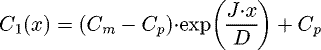
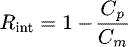
In this work, dead-end filtration was applied to the nanofiltration of synthetic ionic solutions. In order to study the phenomenon of polarization in the boundary layer, we chose NaCl, CaCl2 and Na2(SO4) solutions to pH = 6.8 which concentrations varies from 0.3 to 1.5 g L−1 and the filtration pressure varied from 6 to 16 bar. In this study, the results of these experiments show a correlation between the initial concentration of the solution and the pressure applied with the polarization. The polarization intensifies for the high concentrations and pressures. The ionic balance between the microscopic zone of polarization and the macroscopic state of the solution is described by the following key equation of the model:

The novelty of this model that it is sufficient to know the conductivity and volume flow of permeate solution to calculate precisely the polarization concentration at the membrane surface, the thickness of the polarization layer and the concentration profile inside the boundary layer polarization. It is important to note that the model developed does not take into account the clogging phenomenon because the experiments were done on low concentration synthetic ionic solutions.
Key words: Nanofiltration / Polarization / New model
© Y. Mdemagh et al., Published by EDP Sciences 2018
 This is an Open Access article distributed under the terms of the Creative Commons Attribution License (http://creativecommons.org/licenses/by/4.0/), which permits unrestricted use, distribution, and reproduction in any medium, provided the original work is properly cited.
Introduction
Since the advent of membranes, many studies that date back to 1970 have first aimed at improving the comprehension of the phenomenon involved in the clogging, in more or less short term, to be able to anticipate it, even to control it. Different processes have been used for this purpose: one of the most important is nanofiltration [1–8], which is applied as a means of water treatment in several areas [9–14], such as electrochemical peroxidation [15,16] and electrocoagulation [17] based on different methods.
These efforts are aimed, on the one hand to identify the elements responsible for clogging, on the other hand, to propose methods of quantification leading to provide indications for improving the conduct of operations. In this context, our study of Master's degree focuses on the first clogging step: it is the phenomenon of polarization.
In this case, the main objectives of this research are: (i) the studying of the experimental parameters on a locale scale and their influence on the phenomenon of polarization and (ii) the creation of a new mathematical model by the characterization of the polarization that can be considered as a simple model; which does not require several experimental parameters or sophisticates materials to start it, contrary to others models [18–22] which are sometimes a bit complicated.
Material and methods
This work was focalized on application of the dead-end filtration to the nanofiltration of synthetic ionic solutions such as NaCl, CaCl2 and Na2SO4 at different concentrations (0.3, 0.6, 0.9, 1.2, and 1.5) g L−1 and the filtration pressure varied from 6 to 16 bar. The dead-end filtration experiments were conducted in a laboratory-constructed magnetically stirred cell in dead-end filtration mode. The volume of the cell and the pH of the solution are respectively 200 mL and 6.8. It could be fitted within the module, with an effective membrane surface area of 38.46 cm2. The membrane used is a UTC-80 (ultra-thin composite) from TORAY.
The membrane is conditioned by the filtration of pure water at the progressive pressure in stages of 20 minutes before the tests. The permeability of the membrane is equal to 0.407 L h−1m−2 bar−1 (Fig. 1).
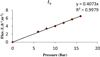 |
Fig. 1 The permeability coefficient of the membrane UTC-80. |
Procedure of the experiment
-
Fill 200 mL of the solution into the separation module and adjust the pressure to 6 bar.
-
Wait 20 min before the first measurement.
-
Collect 5 mL of permeate, T1 is the time necessary to obtain this volume of permeate, the time of the experiment t1 (mn) = 20 + T1.
-
Measure the conductivity of the permeate solution and calculate the Cr1 concentration of the retentate solution with equation (4).
-
Without changing the initial solution, set the pressure to the next value of 8 bar and collect 5 mL of permeate, note also T2 and t2 = 20 + T1 + T2.
-
Measure its conductivity and calculate the Cr2 concentration of the retentate solution.
-
Continue with the same procedure up to 16 bar.
-
Fill a new solution of different concentration and repeat the same procedure.
Modelization of concentration polarization
It should be noticed that in this case, stationary phase cannot be established, and the thickness polarization layer increases from the continuous upcoming ions to theoretically it means the infinity.
Spatial and temporary study of concentration polarization
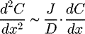
The transport equation for species i corresponds to difference between convection upcoming and diffusion departure.
 (1)
(1)
Fick's second law predicts how the diffusion causes the concentration change with time. It is a one-dimensional partial differential equation:
 (2)
(2)
Equations (1) and (2) can describe the relation of diffusion concentration in terms of time and spatial differentials:
 (3)
(3)
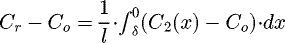
After measuring the concentration of the permeate, it will be possible to know indirectly the concentration of the retentate in the module by mass balance:
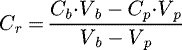 (4)
(4)
The filtration of retentate solution Cr was applied by varying pressure after every 5 mL:
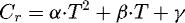 (5)
α, β and γ are constants which are determined from Figure 2. T is the periodic time which is needed to obtain 5 mL of permeate under the considered pressure. Experimentally, T can be presented as a secondary variation function of time:
(5)
α, β and γ are constants which are determined from Figure 2. T is the periodic time which is needed to obtain 5 mL of permeate under the considered pressure. Experimentally, T can be presented as a secondary variation function of time:
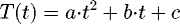 (6)a, b and c are constants which are determined from Figure 3. The variation of the retentate concentration Cr of the solution over time is proportional to the variation of the concentration C(x,t) in the boundary layer's polarization.
The variation of Cr during the experience is illustrated simultaneously from the graphs of Figures 2 and 3.
The concentration depends on two experimental variables: the time t and the periodic time T of filtration:
 (7)
(7)
The resolution of the mass transfer's equation (3) requires the knowledge of the variation of the concentration in the polarization of boundary layer with time. One of the methods to solve this equation is to subdivide the total filtration time t into smaller intervals T and study the polarization phenomenon over the period T. The advantage of this method is to minimize the variation of the concentration over time, it will be shown later in this paper.
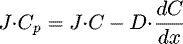
During the filtration, there is a mass accumulation in the polarization of boundary layer. This accumulation will modify the total retentate concentration in the solution. The resulting mass balance is given by the equation below:
 (8)
(8)
Knowing that the function C(x,t) is continuous and bounded on the interval [delta, 0], the integral and the derivative can be permuted:
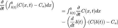 (9)
(9)
With C(δ(t), t) = Co, vx = S ⋅ dx and Vs = S ⋅ l
With equation (8) the result is as follows:
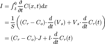 (10)
(10)
The experimental values of each term in this equation are illustrated from Table 1. This table illustrated the minimum and the maximum value.
 (11)
(11)
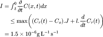
It is important to note that the notion of integral of a function is its algebraic sum on the integration interval; in this case, the derivative of the concentration C(x,t) is positive by the mass accumulation effect.
Therefore, necessarily ∀ xo ∈ [δ, 0]:
 (12)
(12)
For a value from a filtration period T, we have from Table 1 a maximum variation obtained from this equation:
 (13)
(13)
This result proves that 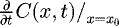 is approximate and is considered as a limited during the interval T. The variation of C(x, t) in time T is negligible.
The problem now is to find a stationary solution for each period T. This leads to the following relation:
 (14)
(14)
Its solution is described as:
 (15)
k1 and k2 are determined under initial conditions:
(15)
k1 and k2 are determined under initial conditions:
 (16)
(16)
 (17)
(17)
Thus
 (18)
(18)
 (19)
(19)
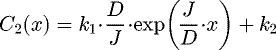
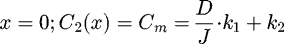
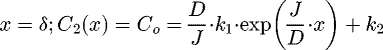
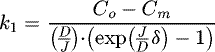
In this case C2 is calculated as:
 (20)
(20)
The convection diffusion of the equilibrium boundary thickness can be described as:
 (21)
C1 is proposed as a solution of this equation:
(21)
C1 is proposed as a solution of this equation:
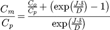
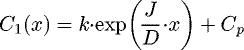 (22)where k is a constant, under the assumed initial conditions x = 0, C(x) = Cm we have:
 (23)
(23)
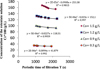 |
Fig. 2 Variation of the retentate concentration as a function of the filtration period T. |
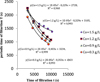 |
Fig. 3 Variation of filtration periodic T as a function of the filtration time t. |
The experimental values.
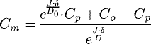
Analytic expression of Cm and δ
Applying initial conditions C1(δ) = Co in equation (23), we got:
 (24)
(24)
According to equation (8) we have:
 (25)
(25)
 (26)
(26)
 (27)
(27)
Assuming the function H as:
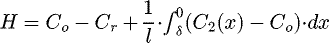 (28)
(28)
For the determination of the expression H, we used software “Maple 18”.
To calculate δ, we need only to impose that H = 0.
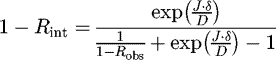
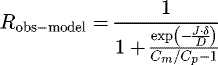
Selectivity expression
We can express (Eq. 24) like as the following relation:
 (29)
(29)
We have also:
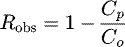 (30)
(30)
 (31)
(31)
This leads to:
 (32)
(32)
Finally, the rejection estimated with the developed model can be written bellow:
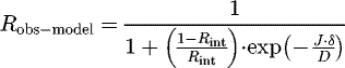 (33)
(33)
 (34)
(34)
Results and discussion
Influence of varying the common ion concentration on process parameters
Flux
For each synthetic solution, the variation of the flux in different pressures is reported in Figures 4–6 .
The flux variation is the same for the three ions within investigated concentrations. The flux decreases proportionally with the concentration by polarization effect.
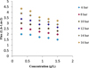 |
Fig. 4 Variation of flux in the case of NaCl. |
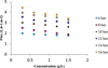 |
Fig. 5 Variation of flux in the case of Na2SO4. |
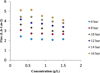 |
Fig. 6 Variation of flux in the case of CaCl2. |
Permeability
Since the hydraulic permeability is an intrinsic specificity of the membrane, we calculated this parameter for all investigated ions with different concentrations. Figure 7 shows that the permeability of CaCl2 is higher than those of NaCl and Na2SO4. This is because of the charge's influence of NF membrane is considered [23], which is confirmed with previous results given by Eriksson and Tsuru et al. [24,25]. The little decreasing of permeability can be explained by the interface polarization effect.
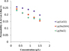 |
Fig. 7 Variation of permeability with different concentration of salts. |
Polarization
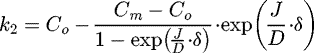
Thickness of the boundary layer polarization (δ)
Using the developed numerical model, we have determined in the case of CaCl2, the effect of varying pressures and concentrations on the thickness of the boundary layer's polarization (δ).
It is clear in Figure 8, with the increasing of the pressure's values during filtration cycle for a given concentration, δ increases until attending a limit value. This is mainly due to the ion accumulation on polarization layer. These observations can be explained by the existence of two types of interactions: van Der Waals attraction interaction (VDW) (varying as 1/r6) and electrostatic attractive interaction (which dependent on 1/r).
Knowing that the energy of electrostatic interaction decreases exponentially as a function of the ionic strength (µ) of the solution, it allows us to understand that at the highest concentrations these interactions are the weakest so the polarization layer will be more compressible, in addition to the VDW attraction interactions will be stronger in this case since the chemical entities will be closer to each other, hence the values of δ at low concentrations will be greater. Chaabane et al. confirmed these results [26]. The limited values of δ for higher pressures were related to repulsive interaction created by the electronic orbital of the chemical entities (energy of Pauli) that have an important gradient (varying as 1/r12) operating on closely distance.
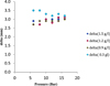 |
Fig. 8 Variation of delta versus Co and P. |
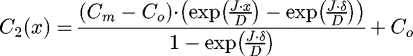
Polarization concentration Cm
The developed model allows us also to calculate polarization concentration Cm and its variation like it is illustrated in Figure 9.
The Cm variation and the flux are in liner regression, as predicted, it increases with higher pressure and concentration. That can be explained by the importance of ion accumulation on the membrane surface.
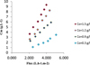 |
Fig. 9 Variation of Cm versus Co and flux. |
Concentration profile on the boundary layer polarization
Knowing the polarization concentration Cm and the thickness δ, and taking to account the equations (5) and (10), we can determine the CaCl2 concentration on the polarization's boundary layer.
Pressure effect
The profiles of the concentrations in the polarization boundary layer are larger for the higher pressures; phenomenon is due to the fact that more pressure is important more the flow is high, and therefore the accumulation of particles will be the biggest (Fig. 10).
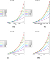 |
Fig. 10 Influence of pressure on spatial distribution of the solution concentration on the polarization boundary layer: (a) Co = 0.3 g L−1, (b) Co = 0.9 g L−1, (c) Co = 1.2 g L−1, and (d) Co = 1.5 g L−1. |
Concentration effect
In this case, pressure is maintained constant while initial concentrations Co are varying (Fig. 11).
The concentration profile in the polarization's boundary layer influences the variation of Cm for higher pressures applied for different initial concentrations. The same effect is observed as that of the case of pressure, for the highest initial concentrations we notice an increase in the concentration profile.
These results have been confirmed by several studies; Chaabane et al. [26] found the same profile of the concentration profile in the polarization boundary layer for several salts and that the polarization concentration increased when the pressure increased. Déon et al. [27] investigated the effect of increasing concentration and pressure on the membrane charge density as well as on the pores and found that the polarization phenomenon was amplified.
The main advantage of this model is its simplicity to describe these phenomena with the knowledge of the initial concentrations in the solutions and the applied pressures. It can be shown that the obtained concentration profile is considered as the result between convection and retro-diffusion of ions.
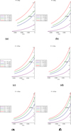 |
Fig. 11 Influence of initial concentration on spatial distribution concentration on the boundary layer polarisation (a) 6 bar, (b) 8 bar, (c) 10 bar, (d) 12 bar, (e) 14 bar, and (f) 16 bar. |
Highlighting of the mass transfer rate by convection and backscattering
It is all perfectly clear that the convective mass transfer is much higher than the transfer by backscattering, otherwise each particle arriving at the membrane surface broadcasts immediately in the heart of the solution and we would have no accumulation of material, so the polarization phenomenon would disappear. To observe the backscattering material transfer effect on the polarization, it is necessary to decrease the transfer convection rate compared to backscattering. For this, the maximum applied pressure will be (16 bar) tolerated by our module at the beginning of material transfer, and then this pressure will gradually decrease up to 6 bar. The evolution of experimental length's boundary layer δ and concentration polarization Cm are illustrated in Figures 12 and 13.
Knowing Cm and δ we can be acquainted with the evolution of the profile's solution concentration in the polarization boundary layer (Figure 14).
During the pressure reduction, the evolution of δ indicates that the latter continues to increase. In addition, the concentration polarization Cm increases proportionally when the pressure fluctuates between 16 and 14 bar. Thereafter, it continues to decline with decreasing pressure.
The evolution of Cm and δ affect directly the concentration profile in the polarization layer. Besides, based on Figure 14, we found that the value of the concentration within the boundary layer Cx grows from 16 to 10 bar and decreases from 8 to 6 bar.
We can say that these phenomena made by fact of applying a pressure equal 16 bar, we compressed the maximum δ boundary layer length which is equal to 1.7 mm and convective transfer is at its maximum. By decreasing the pressure, we will reduce the convective transfer; also, it is even more important than the transfer by backscatter and this is why Cm and δ continue to increase. From 12 bar, the mass transfer phenomenon will change the direction of variation; it is the balance transfer between the phenomenon of convection and diffusion.
At 10 bar, the transfer by backscattering slightly exceeds than the convection. We found that the concentration polarization decreases while δ continues to increase. It may also be noted that from 8 bar, Cm decreases and δ continues to increase when the transfer by backscattering becomes very important, besides of convection, indeed each particle arriving within the boundary layer will be transferred in the heart of the solution and its transfer's speed is proportional to the transferring and the diffusion. Subsequently, the concentration Cx within the boundary layer decreases progressively when the pressure P declines. This is confirmed in Figure 14, when the growth of concentration Cx profile was reported P = 8–6 bar.
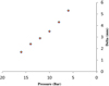 |
Fig. 12 Effect of decreasing of pressure on delta. |
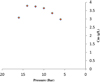 |
Fig. 13 Effect of decreasing the pressure on Cm. |
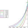 |
Fig. 14 Concentration profile in the polarization boundary layer of the CaCl2 solution at 0.6 g L−1 with decreasing variation of the pressure. |
Model validation: comparative study
Theoretical salts rejections were calculated by equations (30) and (34), by using estimated δ and Cm. Figure 15 shows a comparison between the model's predictions and the experimental results at different concentrations. The figures show that there is an excellent agreement between experimental data and theoretical calculated rejection using our model.
The Figure 16 shows the zones of variations of the retention rate according to equation (34) where Robs is a function of delta and Cm (this figure was obtained using the software “TableCurve 3D v4.0”). Indeed for the low values of Cm the most important retention rates have been reported, but there is a reduction in retention rates when the phenomenon of polarization is important.
 |
Fig. 15 Comparison between predicted and experimental values of the rejection rates. |
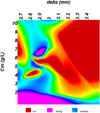 |
Fig. 16 Variation of the retention rate R versus Cm and delta. |
Conclusion
This paper focused on the application of the dead-end filtration on nanofiltration membrane of synthetic ionic solutions. The phenomenon of polarization in the boundary layer and pressure effects were investigated. In this study, a new model has been established that allows determining the thickness of the polarization's boundary layer (δ) and the concentration of polarization (Cm) at the membrane–solution interface.
It allowed us to determine the mathematical expression of the concentration profile in the polarization's boundary layer (Cx). Applying this model to the CaCl2 solution, we were able to follow during the filtration the variation of the concentration profile in the polarization's boundary layer versus the applied pressure and the initial concentration of the solution. This made possible the identification of the mass transfer rate by convection and by retro-diffusion also to follow the evolution of polarization parameters due to the competition between the two phenomena. Finally, this model was validated for the comparison between the experimental retention rates data and the computed one.
List of symbols
Co: Concentration of ionic solution (g L−1)
Cb: Bulk concentration (g L−1)
Cr: Concentration of the retentate solution (g L−1)
Cp: Concentration of the permeate solution (g L−1)
Cx: Concentration profile in the boundary layer polarization
Cm: Concentration of polarization (g L−1)
vx: Elementary volume corresponding to the concentration Cx (m3)
Vs: Volume of solution (m3)
δ: Thickness of the boundary layer polarization (m)
j: Mass flow (g h−1 m−2)
J: Volume flow (L h−1 m−2)
D: Diffusion coefficient (m2 s−1)
t: Total filtration time (s)
T: Filtration period time (s)
l: Depth of the solution in the filtration module (m)
x: Distance to the membrane surface (m)
Robs: Retention rate observed
Rint: Retention rate intrinsic
Lp: Permeability (L h−1 m−2 bar−1)
k: Constant
α: Constant
β: Constant
γ: Constant
a: Constant
b: Constant
c: Constant
k1: Constant
k2: Constant
References
- Mulder M (1997) Basic Principles of Membrane Technology, 2nd ed., Kluwer Academic Publishers, Netherlands. [Google Scholar]
- Rosa MJ, de Pinho MN (1994) Separation of organic solutes by membrane pressure-driven processes. J Membr Sci 89, 235–243. [CrossRef] [Google Scholar]
- Nystrom M, Kaipia L, Luque S (1995), Fouling and retention of nanofiltration membranes. J Membr Sci 98, 249–262. [CrossRef] [Google Scholar]
- Rosa MJ (1995), Separaçao Selectiva de Compostos Organicos de Correntes Aquosas por Ultrafiltraçao e Nanofiltraçao, PhD Thesis, Universidade Tecnica de Lisboa, Instituto Superior Tecnico, Lisboa. [Google Scholar]
- Chaufer B, Baudry-Rabiller M, Guihard L, Daufin G (1996) Retention of ions in nanofiltration at various ionic strength. Desalination 104, 37–46. [CrossRef] [Google Scholar]
- Schaep J, Van der Bruggen B, Vandecasteele C, Wilms D (1998), Influence of ion size and charge in nanofiltration. Separ Purif Technol 14, 155–162. [CrossRef] [Google Scholar]
- Peeters JMM, Mulder MHV, Strathmann H (1999) Streaming potential measurements as a characterization method for nanofiltration membranes. Colloids Surf A: Physicochem Eng Aspects 150, 247–259. [CrossRef] [Google Scholar]
- Childress AE, Elimelech M (2000) Relating nanofiltration membrane performance to membrane charge (electrokinetic) characteristics. Environ Sci Technol 34, 3710–3716. [CrossRef] [Google Scholar]
- Costa AR, de Pinho MN (2006), Performance and cost estimation of nanofiltration for surface water treatment in drinking water production. Desalination 196, 55–65. [CrossRef] [Google Scholar]
- Paugam L, Taha S, Cabon J, Dorange G (2003), Elimination of nitrate ions in drinking waters by nanofiltration. Desalination 152, 271–274. [CrossRef] [Google Scholar]
- Hilal N, Al-Zoubi H, Mohammad AW, Darwish NA (2005) Nanofiltration of highly concentrated salt solutions up to seawater salinity. Desalination 184, 315–326. [CrossRef] [Google Scholar]
- Lhassani A, Rumeau M, Benjelloun D, Pontie M (2001) Selective demineralization of water by nanofiltration application to the defluorination of brackish water. Water Res 35, 3260–3264. [CrossRef] [PubMed] [Google Scholar]
- Van der Bruggen B, Vandecasteele C (2003), Removal of pollutants from surface water and groundwater by nanofiltration: overview of possible applications in the drinking water industry. Environ Pollut 122, 435–445. [CrossRef] [PubMed] [Google Scholar]
- Hilal N, Al-Zoubi H, Darwish NA, Mohammad AW, Abu Arabi M (2004), A comprehensive review of nanofiltration membranes: treatment, pretreatment, modelling, and atomic force microscopy. Desalination 170, 281–308. [CrossRef] [Google Scholar]
- Ahmadzadech S, Dolatabadi M (2018) Modeling and kinetics study of electrochemical peroxidation process for mineralization of bisphenol A; a new paradigm for groundwater treatment. J Mol Liquids 254, 76–82. [CrossRef] [Google Scholar]
- Ahmadzadech S, Dolatabadi M (2018) In situ generation of hydroxyl radical for efficient degradation of 2,4-dichlorophenol from aqueous solutions. Environ Monit Assess 190, 340. [CrossRef] [PubMed] [Google Scholar]
- Ahmadzadech S, Asadipour A, Yoosefian M, Dolatabadi M (2017) Improved electrocoagulation process using chitosan for efficient removal of cefazolin antibiotic from hospital wastewater through sweep flocculation and adsorption : kinetic and isotherm study. Desalin Water Treat 92, 160–171. [CrossRef] [Google Scholar]
- Van der Bruggen B, Manttari M, Nystrom M (2008), Drawbacks of applying nanofiltration and how to avoid them: a review. Sep Purif Technol 63, 251–263. [CrossRef] [Google Scholar]
- Krishna R, Wesselingh JA (1997) The Maxwell-Stefan approach to mass transfert. Chem Eng Sci 52, 861–911. [CrossRef] [Google Scholar]
- Spiegler KS, Kedem O (1966) Thermodynamics of hyperfiltration (reverse osmosis): criteria for coefficient membranes. Desalination 1, 311–326. [CrossRef] [Google Scholar]
- Wang XL, Tsuru T, Nakao S, Kimura S (1995) Electrolyte transport through nanofiltration membranes by the space-charge model and the comparison with Teorell-Meyer-Sievers model. J Membr Sci 103, 117–133. [CrossRef] [Google Scholar]
- Shang W-J, Wang X-L, Yu Y-X (2006), Theoretical calculation on the membrane potential of charged porous membranes in 1-1, 1-2, 2-1 and 2-2 electrolyte solutions. J Membr Sci 285, 362–375. [CrossRef] [Google Scholar]
- Donnan F (1995), Theory of membrane equilibria and membrane potentials in the presence of non-dialysing electrolytes. J Membr Sci 100, 45–55. [CrossRef] [Google Scholar]
- Eriksson P (1988), Nanofiltration extends the range of membrane filtration. Environ Prog 7, 58–62. [CrossRef] [Google Scholar]
- Tsuru T, Urairi M, Nakao SI, Kimura S (1991) Negative rejection of anions in the loose reverse osmosis separation of mono-and divalent ion mixtures. Desalination 81, 219–227. [CrossRef] [Google Scholar]
- Chaabane T, Taha S, Ahmed TM, Maachi R, Dorange G (2007) Coupled model of film theory and the Nernst-Planck equation in nanofiltration. Desalination 206, 424–432. [CrossRef] [Google Scholar]
- Déon S, E scoda A, Fievet P (2011) A transport model considering charge adsorption inside pores to describe salts rejections by nanofiltration membranes. Chem Eng Sci 66, 2823–2832. [CrossRef] [Google Scholar]
Cite this article as: Mdemagh Y, Hafiane A, Ferjani E. (2018), Characterization and modeling of the polarization phenomenon to describe salt rejection by nanofiltration. 4open, 1, 5.
All Tables
All Figures
|
Fig. 1 The permeability coefficient of the membrane UTC-80. |
| In the text | |
|
Fig. 2 Variation of the retentate concentration as a function of the filtration period T. |
| In the text | |
|
Fig. 3 Variation of filtration periodic T as a function of the filtration time t. |
| In the text | |
|
Fig. 4 Variation of flux in the case of NaCl. |
| In the text | |
|
Fig. 5 Variation of flux in the case of Na2SO4. |
| In the text | |
|
Fig. 6 Variation of flux in the case of CaCl2. |
| In the text | |
|
Fig. 7 Variation of permeability with different concentration of salts. |
| In the text | |
|
Fig. 8 Variation of delta versus Co and P. |
| In the text | |
|
Fig. 9 Variation of Cm versus Co and flux. |
| In the text | |
|
Fig. 10 Influence of pressure on spatial distribution of the solution concentration on the polarization boundary layer: (a) Co = 0.3 g L−1, (b) Co = 0.9 g L−1, (c) Co = 1.2 g L−1, and (d) Co = 1.5 g L−1. |
| In the text | |
|
Fig. 11 Influence of initial concentration on spatial distribution concentration on the boundary layer polarisation (a) 6 bar, (b) 8 bar, (c) 10 bar, (d) 12 bar, (e) 14 bar, and (f) 16 bar. |
| In the text | |
|
Fig. 12 Effect of decreasing of pressure on delta. |
| In the text | |
|
Fig. 13 Effect of decreasing the pressure on Cm. |
| In the text | |
|
Fig. 14 Concentration profile in the polarization boundary layer of the CaCl2 solution at 0.6 g L−1 with decreasing variation of the pressure. |
| In the text | |
|
Fig. 15 Comparison between predicted and experimental values of the rejection rates. |
| In the text | |
|
Fig. 16 Variation of the retention rate R versus Cm and delta. |
| In the text | |